# Box plot
## Microsim
### Live player
<div class="microsim-player">
<iframe src="https://editor.p5js.org/sciencenibber/full/hL85l5kZA" width="100%" height="620" frameborder="0" sandbox="allow-scripts allow-same-origin"></iframe>
</div>
<div class="microsim-fallback">
<img src="Microsims/thumbs/Box_plot.png" alt="Box_plot microsim poster" style="width:100%;border:1px solid #4445;border-radius:6px;">
<p><em>Live microsim (desktop) · <a href="https://editor.p5js.org/sciencenibber/sketches/hL85l5kZA">open sketch in the p5.js editor</a></em></p>
</div>
**Editor URL:** https://editor.p5js.org/sciencenibber/sketches/hL85l5kZA
**Description (100 words):**
This Tukey box-and-whisker microsim renders one resistant five-number summary per category — minimum, Q1, median, Q3, maximum — with the IQR as the shaded box, whiskers reaching to the most extreme value within 1.5 × IQR of each quartile, and any further point plotted as an open red outlier. Four built-in datasets (Synthetic, Heights, Reaction-time, Fisher's Iris sepal length) demonstrate uniform, normal, skewed, bimodal, and outlier-heavy shapes side-by-side. Hover any box for an inline numeric readout; toggle a jittered strip-plot of the underlying points, or [[Force|force]] the y-axis to include zero, from the right-side controls. Pure Pattern A composition: chart frame plus glyphBoxplot.
```js
// =====================================================================
// Box_plot.js — Wikitube Visualization microsim
// ---------------------------------------------------------------------
// Slug : Box_plot
// Room : Visualization (the V in GENERATIVE)
// Pattern : Pattern A reskin — Statistical chart types as composition
// (chart frame + scale closures + glyph dictionary entry).
//
// WHAT THIS SKETCH SHOWS
// ----------------------
// Five numeric distributions are summarised side-by-side as Tukey
// box-and-whisker glyphs:
//
// | o <- outlier (beyond 1.5 * IQR)
// |
// +-----+ <- upper whisker (max within 1.5 * IQR)
// | |
// +--+-----+--+ <- box: Q1 to Q3, line at the median
// | | |
// +-----+-----+
// |
// +-----+ <- lower whisker (min within 1.5 * IQR)
// |
// | o <- outlier
//
// The reader can:
// * pick a dataset (Synthetic, Heights, Reaction-time, Iris)
// * toggle the underlying raw points on/off as a strip plot
// * toggle whether the y-axis starts at zero
// Hovering a box surfaces a tooltip with the five-number summary
// and the count of outliers.
//
// PARAMETERS
// ----------
// dataset select which sample to render
// showPoints checkbox overlay raw points as a jittered strip
// zeroBase checkbox force y-axis to include 0
//
// HUD (Betterfire Standard §15)
// -----------------------------
// Top-left : ARTICLE name + en.wikitube.io/wiki/{ARTICLE}
// Top-right : control hint
// Bottom-left: five-number readout for the hovered box
// Bottom-right: equation IQR = Q3 - Q1, fence = 1.5 * IQR
// =====================================================================
const ARTICLE = "Box_plot";
p5.disableFriendlyErrors = true;
// Visualization-room palette (P5_JS_EDITOR.md section 11).
const BG = 250, FG = 24;
const AXIS = [80, 90, 110], GRIDC = [200, 205, 215];
const INK = [40, 48, 60], MUTED = [140, 150, 165];
// Box fill / stroke / accent for an outlier.
const BOX_FILL = [180, 205, 230], BOX_EDGE = [50, 90, 140];
const HI_FILL = [240, 200, 150], HI_EDGE = [200, 110, 40];
const OUTLIER = [200, 60, 60];
const MARGIN = { top: 60, right: 200, bottom: 70, left: 80 };
// ---------------------------------------------------------------------
// DATASETS
// Each dataset is an object { name, yLabel, categories: [{label, vals}] }
// Values are deterministic (fixed seed) so the sketch is reproducible.
// ---------------------------------------------------------------------
let DATASETS;
let datasetSel, pointsCb, zeroCb;
let hoverIdx = -1;
function setup() {
// p5 sets canvas to fixed pixel size; inner layout adapts.
createCanvas(windowWidth, windowHeight);
textFont("system-ui");
textAlign(LEFT, TOP);
randomSeed(11); // reproducible jitter and synthetic data
DATASETS = buildDatasets();
// ---- DOM controls (right-edge column at x = width - 180) -----------
const cx = width - 180;
createDiv("dataset").position(cx, 64).style("color", "#333").style("font-size", "12px");
datasetSel = createSelect();
for (const d of DATASETS) datasetSel.option(d.name);
datasetSel.position(cx, 84).size(160);
pointsCb = createCheckbox(" show raw points", false);
pointsCb.position(cx, 124).style("color", "#333").style("font-size", "12px");
zeroCb = createCheckbox(" force y-axis to 0", false);
zeroCb.position(cx, 148).style("color", "#333").style("font-size", "12px");
}
function draw() {
background(BG);
// 1. Read all controls into named locals at the top of draw —
// the rest of the function is a pure render of these values.
const ds = DATASETS.find(d => d.name === datasetSel.value()) || DATASETS[0];
const showPts = pointsCb.checked();
const zeroBase = zeroCb.checked();
// 2. Compute the chart's pixel rectangle.
const x0 = MARGIN.left, y0 = MARGIN.top;
const w = width - MARGIN.left - MARGIN.right;
const h = height - MARGIN.top - MARGIN.bottom;
// 3. Compute summaries for every category once per frame. Cheap.
const summaries = ds.categories.map(c => fiveNumber(c.vals));
// 4. Y-domain: pad the global min/max by 5%, optionally clip to [0,_].
let lo = Math.min(...summaries.map(s => s.lo));
let hi = Math.max(...summaries.map(s => s.hi));
// include outlier extremes too:
for (const s of summaries) {
for (const o of s.outliers) { lo = Math.min(lo, o); hi = Math.max(hi, o); }
}
const pad = (hi - lo) * 0.06 || 1;
let yLo = lo - pad, yHi = hi + pad;
if (zeroBase) yLo = Math.min(0, yLo);
// 5. Scale closures (chart_frame.js style).
// xScale takes a category index, yScale takes a data value.
const xScale = (i) => x0 + (i + 0.5) * (w / ds.categories.length);
const yScale = (v) => y0 + h - ((v - yLo) / (yHi - yLo)) * h;
const bandW = (w / ds.categories.length);
const boxW = bandW * 0.5; // box half-width is boxW/2 either side
// 6. Frame: gridlines, axes, ticks, axis titles, chart title.
drawFrame(x0, y0, w, h, ds, yLo, yHi);
// 7. Hover detection: which box is the mouse over?
hoverIdx = -1;
for (let i = 0; i < ds.categories.length; i++) {
const cx = xScale(i);
if (mouseX > cx - boxW / 2 && mouseX < cx + boxW / 2 &&
mouseY > y0 && mouseY < y0 + h) {
hoverIdx = i;
break;
}
}
// 8. Paint a strip-plot of raw points behind the box if requested —
// Tukey himself recommended this for small N.
if (showPts) {
noStroke();
for (let i = 0; i < ds.categories.length; i++) {
const cx = xScale(i);
fill(MUTED[0], MUTED[1], MUTED[2], 130);
for (const v of ds.categories[i].vals) {
// deterministic horizontal jitter via a tiny hash on v
const jitter = ((Math.sin(v * 12.9898) * 43758.5453) % 1) * (boxW * 0.6);
circle(cx + jitter - boxW * 0.3, yScale(v), 4);
}
}
}
// 9. Glyph emission: one box per category. The whole "box plot" is
// just this loop — Pattern A composition in action.
for (let i = 0; i < ds.categories.length; i++) {
const cx = xScale(i);
const s = summaries[i];
glyphBoxplot(cx, boxW, s, yScale, i === hoverIdx);
// category label centered on tick
noStroke(); fill(AXIS[0], AXIS[1], AXIS[2]);
textSize(11); textAlign(CENTER, TOP);
text(ds.categories[i].label, cx, y0 + h + 10);
}
textAlign(LEFT, TOP);
// 10. HUD overlays (top-left identity, top-right hint,
// bottom-left readout, bottom-right equation).
drawHud(ds, summaries);
}
// ---------------------------------------------------------------------
// glyphBoxplot — the only visualisation primitive that's specific to
// this article. Everything else (frame, axes, scales) is generic.
//
// Inputs in DATA coordinates:
// s = { lo, q1, q2, q3, hi, outliers }
// Inputs in PIXEL coordinates:
// cx = x-pixel of the category centre
// boxW = pixel width of the IQR box
// yScale = closure mapping data y -> pixel y
// hot = boolean, this box is the hovered one
// ---------------------------------------------------------------------
function glyphBoxplot(cx, boxW, s, yScale, hot) {
const yLo = yScale(s.lo);
const yQ1 = yScale(s.q1);
const yMd = yScale(s.q2);
const yQ3 = yScale(s.q3);
const yHi = yScale(s.hi);
const fillC = hot ? HI_FILL : BOX_FILL;
const edgeC = hot ? HI_EDGE : BOX_EDGE;
// whisker stem (vertical from lower to upper fence)
stroke(edgeC[0], edgeC[1], edgeC[2]); strokeWeight(hot ? 1.6 : 1.2);
line(cx, yLo, cx, yHi);
// whisker caps (short horizontal bars at min and max)
const capW = boxW * 0.5;
line(cx - capW / 2, yLo, cx + capW / 2, yLo);
line(cx - capW / 2, yHi, cx + capW / 2, yHi);
// IQR box (Q1 to Q3)
fill(fillC[0], fillC[1], fillC[2]);
stroke(edgeC[0], edgeC[1], edgeC[2]); strokeWeight(hot ? 1.6 : 1.2);
rect(cx - boxW / 2, yQ3, boxW, yQ1 - yQ3, 2);
// median line — drawn on top of the box for emphasis
stroke(edgeC[0], edgeC[1], edgeC[2]); strokeWeight(hot ? 2.4 : 1.8);
line(cx - boxW / 2, yMd, cx + boxW / 2, yMd);
// outliers as small open circles
noFill(); stroke(OUTLIER[0], OUTLIER[1], OUTLIER[2]); strokeWeight(1.2);
for (const o of s.outliers) circle(cx, yScale(o), 5);
}
// ---------------------------------------------------------------------
// fiveNumber — Tukey's resistant five-number summary plus outliers.
//
// Uses the standard convention:
// Q1, Q2, Q3 are the 25th, 50th, 75th percentiles by linear
// interpolation on the sorted vector (matches numpy default).
// IQR = Q3 - Q1
// fence_lo = Q1 - 1.5 * IQR, fence_hi = Q3 + 1.5 * IQR
// lo = smallest value >= fence_lo, hi = largest value <= fence_hi
// outliers = values outside [fence_lo, fence_hi]
// ---------------------------------------------------------------------
function fiveNumber(values) {
const v = [...values].sort((a, b) => a - b);
const q = (p) => {
const idx = (v.length - 1) * p;
const i = Math.floor(idx), f = idx - i;
return i + 1 < v.length ? v[i] * (1 - f) + v[i + 1] * f : v[i];
};
const q1 = q(0.25), q2 = q(0.5), q3 = q(0.75);
const iqr = q3 - q1;
const fLo = q1 - 1.5 * iqr, fHi = q3 + 1.5 * iqr;
const inside = v.filter(x => x >= fLo && x <= fHi);
const outliers = v.filter(x => x < fLo || x > fHi);
return {
n: v.length,
q1, q2, q3,
iqr,
lo: inside.length ? inside[0] : q1,
hi: inside.length ? inside[inside.length - 1] : q3,
outliers,
};
}
// ---------------------------------------------------------------------
// drawFrame — gridlines, axes, tick labels, axis titles, chart title.
// This is the chart_frame.js shape that Visualization is supposed to
// factor out — kept inline here so the sketch is self-contained.
// ---------------------------------------------------------------------
function drawFrame(x, y, w, h, ds, yLo, yHi) {
const ticks = niceTicks(yLo, yHi, 6);
// gridlines
stroke(GRIDC[0], GRIDC[1], GRIDC[2]); strokeWeight(1);
for (const t of ticks) {
const yy = y + h - ((t - yLo) / (yHi - yLo)) * h;
line(x, yy, x + w, yy);
}
// axes
stroke(AXIS[0], AXIS[1], AXIS[2]); strokeWeight(1.5);
line(x, y, x, y + h);
line(x, y + h, x + w, y + h);
// y-axis tick labels
noStroke(); fill(AXIS[0], AXIS[1], AXIS[2]);
textAlign(RIGHT, CENTER); textSize(10);
for (const t of ticks) {
const yy = y + h - ((t - yLo) / (yHi - yLo)) * h;
text(formatTick(t), x - 6, yy);
}
// y-axis title (rotated)
push(); translate(x - 50, y + h / 2); rotate(-HALF_PI);
fill(AXIS[0], AXIS[1], AXIS[2]); textAlign(CENTER, CENTER); textSize(12);
text(ds.yLabel, 0, 0); pop();
// chart title
fill(INK[0], INK[1], INK[2]);
textAlign(LEFT, TOP); textSize(14);
text(ds.name + " - Tukey box-and-whisker", x, y - 28);
// restore default text alignment
textAlign(LEFT, TOP);
}
// niceTicks — pick ~k tick values inside [a, b] that look human.
function niceTicks(a, b, k) {
const range = b - a;
if (range <= 0) return [a];
const step = niceStep(range / k);
const start = Math.ceil(a / step) * step;
const out = [];
for (let v = start; v <= b + 1e-9; v += step) out.push(v);
return out;
}
function niceStep(raw) {
const exp = Math.floor(Math.log10(raw));
const f = raw / Math.pow(10, exp);
const nice = f < 1.5 ? 1 : f < 3 ? 2 : f < 7 ? 5 : 10;
return nice * Math.pow(10, exp);
}
function formatTick(v) {
if (Math.abs(v) >= 1000 || (v !== 0 && Math.abs(v) < 0.01)) return v.toExponential(1);
return Number.isInteger(v) ? v.toString() : v.toFixed(2);
}
// ---------------------------------------------------------------------
// drawHud — Wikitube HUD: identity TL, hint TR, readout BL, equation BR.
// ---------------------------------------------------------------------
function drawHud(ds, summaries) {
// identity (top-left)
noStroke(); fill(0, 180);
rect(8, 8, 360, 28, 3);
fill(255); textSize(13); textAlign(LEFT, CENTER);
text(ARTICLE + " . en.wikitube.io/wiki/" + ARTICLE, 16, 22);
// hint (top-right)
textAlign(RIGHT, CENTER); fill(MUTED[0], MUTED[1], MUTED[2]);
textSize(11);
text("hover a box for the 5-number summary",
width - 16, 22);
// readout (bottom-left): hovered box's summary or global
textAlign(LEFT, BOTTOM); fill(INK[0], INK[1], INK[2]); textSize(11);
let line1, line2;
if (hoverIdx >= 0) {
const s = summaries[hoverIdx];
const c = ds.categories[hoverIdx];
line1 = c.label + ": n=" + s.n +
" min=" + formatTick(s.lo) +
" Q1=" + formatTick(s.q1) +
" med=" + formatTick(s.q2) +
" Q3=" + formatTick(s.q3) +
" max=" + formatTick(s.hi);
line2 = "outliers: " + s.outliers.length +
(s.outliers.length ? " values: " +
s.outliers.map(formatTick).join(", ") : "");
} else {
line1 = ds.name + " . " + ds.categories.length + " categories . " +
"total n = " + ds.categories.reduce((a, c) => a + c.vals.length, 0);
line2 = "select a dataset on the right; hover a box to inspect.";
}
text(line1, 14, height - 26);
text(line2, 14, height - 12);
// equation (bottom-right)
textAlign(RIGHT, BOTTOM); fill(MUTED[0], MUTED[1], MUTED[2]); textSize(11);
text("IQR = Q3 - Q1 . fence = 1.5 * IQR",
width - 14, height - 12);
textAlign(LEFT, TOP);
}
// ---------------------------------------------------------------------
// buildDatasets — four built-in samples. Each one demonstrates a
// different shape so the reader can see the box plot's behaviour.
//
// Synthetic : five hand-crafted distributions (uniform, normal,
// skewed, bimodal, with outliers)
// Heights : adult heights in cm by self-reported group (toy)
// Reaction : reaction time in ms by hour-of-day bucket (toy)
// Iris : sepal length in cm by species (the classic 1936
// Anderson / Fisher dataset, three species, n=50 each;
// values rounded to one decimal for compactness)
// ---------------------------------------------------------------------
function buildDatasets() {
// helpers — these run after randomSeed so they're reproducible.
const N = (mu, sd, n) => {
const out = [];
for (let i = 0; i < n; i++) {
// Box-Muller transform
const u1 = random(), u2 = random();
const z = Math.sqrt(-2 * Math.log(u1)) * Math.cos(2 * Math.PI * u2);
out.push(mu + sd * z);
}
return out;
};
const U = (a, b, n) => {
const out = [];
for (let i = 0; i < n; i++) out.push(a + (b - a) * random());
return out;
};
const skew = (n) => U(0, 1, n).map(u => Math.pow(u, 0.4) * 100);
const bim = (n) => Array.from({ length: n },
(_, i) => i % 2 === 0
? 30 + 6 * (random() - 0.5)
: 70 + 6 * (random() - 0.5));
const withOutliers = N(50, 8, 40).concat([5, 95, 100]);
return [
{
name: "Synthetic",
yLabel: "value",
categories: [
{ label: "uniform", vals: U(20, 80, 40) },
{ label: "normal", vals: N(50, 10, 40) },
{ label: "skewed", vals: skew(40) },
{ label: "bimodal", vals: bim(40) },
{ label: "outliers", vals: withOutliers },
],
},
{
name: "Heights (cm)",
yLabel: "height (cm)",
categories: [
{ label: "group A", vals: N(165, 6, 30) },
{ label: "group B", vals: N(172, 7, 30) },
{ label: "group C", vals: N(178, 8, 30) },
],
},
{
name: "Reaction time (ms)",
yLabel: "RT (ms)",
categories: [
{ label: "morning", vals: N(280, 35, 30) },
{ label: "afternoon", vals: N(255, 30, 30) },
{ label: "evening", vals: N(310, 45, 30).concat([520, 540]) },
],
},
{
// Iris sepal length by species — Fisher 1936, rounded to 1 dp.
// Source: UCI Machine Learning Repository / Anderson 1935.
name: "Iris (sepal length)",
yLabel: "sepal length (cm)",
categories: [
{ label: "setosa", vals: [
5.1,4.9,4.7,4.6,5.0,5.4,4.6,5.0,4.4,4.9,
5.4,4.8,4.8,4.3,5.8,5.7,5.4,5.1,5.7,5.1,
5.4,5.1,4.6,5.1,4.8,5.0,5.0,5.2,5.2,4.7,
4.8,5.4,5.2,5.5,4.9,5.0,5.5,4.9,4.4,5.1,
5.0,4.5,4.4,5.0,5.1,4.8,5.1,4.6,5.3,5.0,
]},
{ label: "versicolor", vals: [
7.0,6.4,6.9,5.5,6.5,5.7,6.3,4.9,6.6,5.2,
5.0,5.9,6.0,6.1,5.6,6.7,5.6,5.8,6.2,5.6,
5.9,6.1,6.3,6.1,6.4,6.6,6.8,6.7,6.0,5.7,
5.5,5.5,5.8,6.0,5.4,6.0,6.7,6.3,5.6,5.5,
5.5,6.1,5.8,5.0,5.6,5.7,5.7,6.2,5.1,5.7,
]},
{ label: "virginica", vals: [
6.3,5.8,7.1,6.3,6.5,7.6,4.9,7.3,6.7,7.2,
6.5,6.4,6.8,5.7,5.8,6.4,6.5,7.7,7.7,6.0,
6.9,5.6,7.7,6.3,6.7,7.2,6.2,6.1,6.4,7.2,
7.4,7.9,6.4,6.3,6.1,7.7,6.3,6.4,6.0,6.9,
6.7,6.9,5.8,6.8,6.7,6.7,6.3,6.5,6.2,5.9,
]},
],
},
];
}
function windowResized() { resizeCanvas(windowWidth, windowHeight); }
```
## Links (Wikipedia order)
<!-- injected from _registry/childlinks/Box_plot.json (2026-07-30T02:09:12Z) -->
`Accelerated_failure_time_model` · `Actuarial_science` · `Addison-Wesley` · `Akaike_information_criterion` · `Analysis_of_covariance` · `Analysis_of_variance` · `Anderson–Darling_test` · `Anscombe_transform` · `Arithmetic_mean` · `Arithmetic–geometric_mean` · `Asymptotic_theory_(statistics)` · [[Autocorrelation]] · `Autoregressive_conditional_heteroskedasticity` · `Autoregressive_model` · `Average_absolute_deviation` · `Bagplot` · [[Bar_chart]] · `Bayes_estimator` · `Bayes_factor` · `Bayesian_inference` · `Bayesian_information_criterion` · `Bayesian_linear_regression` · `Bayesian_probability` · `Bias_of_an_estimator` · `Binomial_regression` · [[Bioinformatics]] · `Biostatistics` · `Biplot` · `Blocking_(statistics)` · `Bootstrapping_(statistics)` · `Box–Jenkins_method` · `Breusch–Godfrey_test` · `Canonical_correlation` · `Cartography` · `Categorical_variable` · `Census` · `Central_limit_theorem` · `Chemometrics` · `Chi-squared_test` · `Clinical_study_design` · `Clinical_trial` · `Cluster_analysis` · `Cluster_sampling` · `Cochran–Mantel–Haenszel_statistics` · `Coefficient_of_determination` · `Coefficient_of_variation` · `Cohen's_kappa` · `Cohort_study` · `Cointegration` · `Completeness_(statistics)` · `Confidence_interval` · `Confounding` · `Contingency_table` · `Contour_boxplot` · `Contraharmonic_mean` · `Control_chart` · `Correlogram` · `Count_data` · `Credible_interval` · `Crime_statistics` · `Cross-correlation` · `Cross-sectional_study` · `Cross-validation_(statistics)` · `Cubic_mean` · `Data_and_information_visualization` · `Data_collection` · `Data_preprocessing` · `Data_transformation_(statistics)` · `Decomposition_of_time_series` · `Degrees_of_freedom_(statistics)` · `Demographic_statistics` · `Density_estimation` · `Descriptive_statistics` · `Design_of_experiments` · `Dickey–Fuller_test` · `Dimensionality_reduction` · `Divergence_(statistics)` · `Durbin–Watson_statistic` · `Econometrics` · `Effect_size` · `Efficiency_(statistics)` · `Elliptical_distribution` · `Empirical_distribution_function` · `Engineering_statistics` · `Environmental_statistics` · `Epidemiology` · `Errors_and_residuals` · `Estimating_equations` · `Experiment` · `Exploratory_data_analysis` · `Exponential_family` · `Exponential_smoothing` · `F-test` · `Factor_analysis` · `Factorial_experiment` · `Failure_rate` · `Fan_chart_(statistics)` · `Feature_scaling` · `First-hitting-time_model` · `Fisher_transformation` · `Five-number_summary` · `Forest_plot` · [[Fourier_analysis]] · [[Frequency_domain]] · `Frequentist_inference` · `Friedman_test` · `Functional_boxplot` · `G-test` · `General_linear_model` · `Generalized_linear_model` · `Generalized_mean` · `Geographic_information_system` · `Geometric_mean` · `Geostatistics` · `Goodness_of_fit` · `Granger_causality` · `Graphical_model` · `Grouped_data` · `Harmonic_mean` · `Heinz_mean` · `Heronian_mean` · [[Histogram]] · `Hodges–Lehmann_estimator` · `Homoscedasticity_and_heteroscedasticity` · `Index_of_dispersion` · `Interaction_(statistics)` · `Interquartile_range` · `Interval_estimation` · `Isotonic_regression` · `Jackknife_resampling` · `Jarque–Bera_test` · `Johansen_test` · `John_Tukey` · `Jonckheere's_trend_test` · `Jurimetrics` · `Kaplan–Meier_estimator` · `Kendall_rank_correlation_coefficient` · `Kernel_density_estimation` · `Kolmogorov–Smirnov_test` · `Kriging` · `Kruskal–Wallis_test` · `Kurtosis` · `L-estimator` · `L-moment` · [[Least-squares_spectral_analysis]] · `Lehmann–Scheffé_theorem` · `Lehmer_mean` · `Likelihood-ratio_test` · `Likelihood_function` · `Lilliefors_test` · [[Line_chart]] · `Linear_discriminant_analysis` · `Linear_regression` · `List_of_fields_of_application_of_statistics` · `List_of_statistical_tests` · `List_of_statistics_articles` · `Ljung–Box_test` · `Location_parameter` · `Location–scale_family` · `Logistic_regression` · `Loss_function` · `Lp_space` · `M-estimator` · `Mann–Whitney_U_test` · `Mary_Eleanor_Spear` · `Maximum_a_posteriori_estimation` · `McNemar's_test` · `Medcouple` · `Median` · `Medical_statistics` · `Method_of_moments_(statistics)` · `Methods_engineering` · `Mia_Hubert` · `Michelson–Morley_experiment` · `Mid-range` · `Midhinge` · `Minimum-variance_unbiased_estimator` · `Missing_data` · `Mixed_model` · `Mode_(statistics)` · `Model_selection` · `Moment_(mathematics)` · `Monotone_likelihood_ratio` · `Multimodal_distribution` · `Multivariate_analysis_of_variance` · `Multivariate_normal_distribution` · `Multivariate_statistics` · `National_accounts` · `Natural_experiment` · `Nelson–Aalen_estimator` · `Nonlinear_regression` · `Nonparametric_regression` · `Nonparametric_statistics` · `Normal_distribution` · `Normalization_(statistics)` · `Observational_study` · `Official_statistics` · `One-_and_two-tailed_tests` · `Opinion_poll` · `Optimal_decision` · `Order_statistic` · `Ordinary_least_squares` · `Outlier` · `Outline_of_statistics` · `Parametric_statistics` · `Partial_autocorrelation_function` · `Partial_correlation` · `Partition_of_sums_of_squares` · `Pearson_correlation_coefficient` · `Percentile` · `Permutation_test` · `Peter_Rousseeuw` · `Pie_chart` · `Pivotal_quantity` · `Point_estimation` · `Poisson_regression` · `Posterior_probability` · `Power_(statistics)` · `Power_transform` · `Prediction_interval` · `Principal_component_analysis` · `Prior_probability` · `Probabilistic_design` · [[Probability_density_function]] · `Probability_distribution` · `Proportional_hazards_model` · `Psychometrics` · `Quality_control` · `Quartile` · `Quasi-experiment` · `Questionnaire` · `Q–Q_plot` · `Radar_chart` · `Random_assignment` · `Randomized_controlled_trial` · `Randomized_experiment` · `Range_(statistics)` · `Rank_correlation` · `Ranking_(statistics)` · `Rao–Blackwell_theorem` · `Regression_analysis` · `Regression_validation` · [[Reliability_engineering]] · `Replication_(statistics)` · `Resampling_(statistics)` · `Robust_regression` · `Robust_statistics` · `Run_chart` · `Sample_size_determination` · `Sampling_(statistics)` · `Sampling_distribution` · `Scale_parameter` · [[Scatter_plot]] · `Scientific_control` · `Score_test` · `Seasonal_adjustment` · `Seasonality` · `Semiparametric_regression` · `Seven-number_summary` · `Shape_parameter` · `Shapiro–Wilk_test` · `Sign_test` · `Simple_linear_regression` · `Simultaneous_equations_model` · `Sina_plot` · `Skewness` · `Social_statistics` · `Spatial_analysis` · `Spearman's_rank_correlation_coefficient` · `Spectral_density_estimation` · `Standard_deviation` · `Standard_error` · `Standard_score` · `Stationary_process` · `Statistic` · `Statistical_classification` · `Statistical_dispersion` · `Statistical_distance` · `Statistical_graphics` · `Statistical_hypothesis_test` · `Statistical_inference` · `Statistical_model` · `Statistical_parameter` · `Statistical_population` · `Statistical_process_control` · `Statistical_theory` · `Statistics` · `Stem-and-leaf_display` · `Stochastic_approximation` · `Stratified_sampling` · `Structural_break` · `Structural_equation_modeling` · `Student's_t-test` · `Sufficient_statistic` · `Survey_methodology` · `Survival_analysis` · `Survival_function` · [[System_identification]] · `The_American_Statistician` · [[Time_domain]] · [[Time_series]] · `Tolerance_interval` · `Trimean` · `Truncation_(statistics)` · `U-statistic` · `Uniformly_most_powerful_test` · `V-statistic` · `Van_der_Waerden_test` · `Variance` · `Variance-stabilizing_transformation` · `Vector_autoregression` · `Violin_plot` · `Wald_test` · `Wavelet` · `Whittle_likelihood` · `Wilcoxon_signed-rank_test` · `Winsorizing` · `Z-test`
## From the Real GENERATIVE library
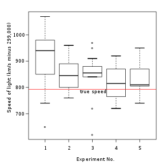
*Box plot — placed from the Real G.E.N.E.R.A.T.I.V.E. course library (Visualization room). Source: Wikimedia Commons (via Wikipedia article media). [Details & license](https://commons.wikimedia.org/wiki/File:Michelsonmorley-boxplot.svg).*
> In descriptive statistics, a box plot or boxplot is a method for demonstrating graphically the locality, spread and skewness groups of numerical data through their quartiles.[1] In addition to the box on a box plot, there can be lines (which are called whiskers) extending from the box indicating variability outside the upper and lower quartiles, thus, the pl ([Wikipedia](https://en.wikipedia.org/wiki/Box_plot))
<!-- REAL-GENERATIVE-MEDIA:END -->
<!-- LOCAL-MEDIA-PASS:START -->
## From the vault media library
!Box plot thumb.png
*Box Plot — from the vault's own media holdings, placed 2026-07-09. MTN / Wikitube.io original · CC BY-SA 4.0.*
<!-- LOCAL-MEDIA-PASS:END -->
> **Room:** Visualization · **Status:** ✅ shipped
## Overview
A **box plot** (or **box-and-whisker plot**) is a non-parametric summary of a numeric distribution that compresses five descriptive statistics — minimum, first quartile (Q1), median (Q2), third quartile (Q3), and maximum — into a single compact glyph. The "box" spans the interquartile range (IQR = Q3 − Q1) and is bisected by a line at the median; "whiskers" extend outward to the smallest and largest values within 1.5 × IQR of the quartiles, and any observation beyond that threshold is plotted as an individual point and read as an **outlier**. The convention was introduced by John Tukey in his 1977 *Exploratory Data Analysis*, where he argued for resistant statistics that survive a single anomalous reading without distorting the picture, and it has since become the default visual for comparing the shapes of several distributions side-by-side. Unlike a [[Histogram|histogram]], the box plot is invariant to bin choice; unlike a mean-with-error-bar, it does not assume Gaussian shape. Its weaknesses are well-known too: a box plot hides multimodality (a violin plot or strip plot is the remedy), and the 1.5 × IQR fence is a heuristic, not a probability claim. The microsim below renders one box per category from a configurable dataset and exposes the underlying points on hover.
## See also
- Room hub: Visualization
- p5.js Editor conventions: P5 JS EDITOR
- Wiki root: MAIN
---
*Scaffolded by `generative-microsim` from row 0 of the Visualization sheet on 2026-04-30T17:51:39Z.*
Letters: mined_visualization · chart_glyph_dictionary · distribution · probability · filter · rotation · sampling · conservation
<!-- REAL-GENERATIVE-MEDIA:START -->
<!-- CRAFT-LINK:START g12 -->
*Built to the [[WT!P5_js_Microsim_Master_Class|p5.js Master Class]].*
<!-- CRAFT-LINK:END -->
## Wikipedia : Wikitube
**Strict pair:** [Wikipedia](https://en.wikipedia.org/wiki/Box_plot) : [Wikitube](https://en.wikitube.io/wiki/Box_plot)
## Previous hub tags
Tree parents: [[Monte_Carlo_method]] · [[Reliability_engineering]].
Legacy hubs: `GENERATIVE`.
---
*Sources: 1 legacy note. Minted wave 1, 2026-07-30 (v1.6 order).*