# Electric current
## Microsim
<iframe src="https://editor.p5js.org/sciencenibber/full/n7H920z5s" width="100%" height="620" frameborder="0" sandbox="allow-scripts allow-same-origin"></iframe>
<img src="../SPINTRONICS Images/Electric_current.png" alt="Electric_current microsim">
*Live sketch: [open in the p5.js editor](https://editor.p5js.org/sciencenibber/sketches/n7H920z5s). The poster image above is a placeholder pending an attended or server-side canvas capture.*
### p5.js source
```js
// Electric_current.js -- Wikitube MicroSim
// Hub: SPINTRONICS · Branch: P - Power transmission
// Pattern: J (particles / agents) -- a sea of charge carriers drifting through a
// conductor. Animation is the point (the swarm drifts), so we loop()
// while playing but keep every per-frame loop bounded (~140 carriers,
// one update pass, no per-pixel work) so the editor's loop-protect is
// never tripped.
//
// CONCEPT
// Electric current is the net drift of a carrier swarm past a cross-section:
// I = dQ/dt = n * q * v_d * A
// with n the carrier number density (m^-3), q the carrier charge (e), v_d the
// drift velocity (m/s), and A the cross-section (m^2). The drift comes from the
// field via the Drude model, v_d = mu*E with mobility mu = q*tau/m, giving the
// microscopic Ohm's law J = n*q*v_d = sigma*E (sigma = 1/rho). For a wire of
// length L the field is E = V/L, and I = sigma*E*A = V/R with R = rho*L/A -- so
// the macroscopic V = I*R falls out of the drifting swarm.
// The "aha": v_d is sub-mm/s even while the random Fermi speed is ~1e6 m/s
// (ratio ~1e10). Carriers barely crawl; the current is still large and steady.
//
// Sign convention (metal): carriers are electrons (q < 0), so they drift
// OPPOSITE the field E; the conventional current I points ALONG E. Both are
// drawn and labelled.
//
// GOLDEN RULES honoured: 720x520 + pixelDensity(2); layout derived from
// width/height; ASCII-only strings (Unicode only in comments); SI units
// internally, convert at the input; dt clamped (min(deltaTime/1000,0.05));
// cheap draw() with a baked offscreen scenery buffer; bounded per-frame loop;
// HUD watermark drawn last; one concept per control; reset restores ALL state;
// p5.disableFriendlyErrors = true.
const ARTICLE = "Electric_current"; // single source of truth (HUD + save + URL)
// ---- physical constants (SI) ----
const ECHARGE = 1.602e-19; // e, coulombs (magnitude of the elementary charge)
const L_WIRE = 0.10; // m, fixed length of the modelled wire segment
// ---- materials: carrier density n (m^-3), resistivity rho (Ohm*m), and an
// approximate random/Fermi speed vF (m/s) used only for the contrast read.
// mobility mu and conductivity sigma are DERIVED so everything stays
// self-consistent: mu = 1/(n*e*rho), sigma = 1/rho, hence J = n*e*v_d = sigma*E.
const MATERIALS = [
{ name: "Copper", n: 8.50e28, rho: 1.68e-8, vF: 1.57e6, col: [255, 150, 80] },
{ name: "Aluminium", n: 1.81e29, rho: 2.65e-8, vF: 2.03e6, col: [180, 200, 230] },
{ name: "Nichrome", n: 9.20e28, rho: 1.10e-6, vF: 1.40e6, col: [230, 120, 120] }
];
// ---- control ranges (real symbols, meaningful ranges) ----
const V_MIN = 0, V_MAX = 25, V_DEF = 10; // V, millivolts (across L = 0.10 m)
const A_MIN = 0.5, A_MAX = 10, A_DEF = 1.0; // A, square millimetres
// ---- visualization scaling (the drift is exaggerated/slowed to be visible) ----
const VIS_GAIN = 2.3e4; // px/s of on-screen drift per (m/s) of real v_d
const THERMAL = 190; // px/s amplitude of the decorative thermal jitter
const NPART = 140; // carrier dots drawn (bounded -> cheap, clean loop)
// ---- controls ----
let vSlider, aSlider;
let materialButton, playButton, resetButton;
// ---- state ----
let matIndex = 0; // index into MATERIALS
let isPlaying = true;
let electrons = []; // {x, y} carrier dots in channel pixel coords
let markerX = 0; // marching "v_d (scaled)" speed marker
let simClock = 0; // s, elapsed sim time for the charge odometer
let qOdo = 0; // C, integrated charge Q = integral(I dt)
let scenery; // baked static buffer (walls, labels, dividers)
// ---- layout (all derived; never hard-code magic coords in draw) ----
let chX0, chX1, chY0, chY1, chMidY, chW; // conductor channel rectangle
let arrowY, fieldY; // conventional-current + field arrow rows
// ---- palette (ASCII identifiers only; none collide with p5 globals) ----
let BG, INK, MUTE, FRAME, WIRE, ECOL, CURR, FIELDC, GOOD;
function setup() {
createCanvas(720, 520);
pixelDensity(2);
p5.disableFriendlyErrors = true; // clean + cheap; no FES overhead
textFont("monospace");
BG = color(14, 18, 32);
INK = color(232, 238, 248);
MUTE = color(120, 134, 158);
FRAME = color(60, 72, 96);
WIRE = color(36, 44, 64); // conductor body
ECOL = color(110, 180, 255); // electron carriers (blue)
CURR = color(120, 230, 150); // conventional-current arrow (green)
FIELDC = color(255, 200, 110); // applied field E (amber)
GOOD = color(120, 230, 150);
// --- geometry from the canvas, not magic numbers ---
chX0 = 60; chX1 = 470; chY0 = 150; chY1 = 250;
chMidY = (chY0 + chY1) / 2; chW = chX1 - chX0;
arrowY = chY0 - 40; // "I ->" row, above the wire
fieldY = chY1 + 34; // "E ->" row, below the wire
buildControls();
initElectrons();
markerX = chX1 - 8; // start the speed marker at the right end
buildScenery(); // bake once -> draw() paints only dynamics
// loop() runs while playing; we start armed and playing
}
function buildControls() {
// one slider per concept, carrying the field's real symbol + a meaningful range
vSlider = createSlider(V_MIN, V_MAX, V_DEF, 1); // V, millivolts
aSlider = createSlider(A_MIN, A_MAX, A_DEF, 0.5); // A, mm^2
vSlider.position(24, 392); vSlider.style("width", "180px");
aSlider.position(24, 430); aSlider.style("width", "180px");
materialButton = createButton("material: Copper");
materialButton.position(24, 470);
materialButton.mousePressed(cycleMaterial);
playButton = createButton("pause");
playButton.position(214, 470);
playButton.mousePressed(togglePlay);
resetButton = createButton("reset");
resetButton.position(288, 470);
resetButton.mousePressed(resetAll);
// changing V or A re-arms the charge odometer so Q/t == I stays exact/clean
vSlider.input(reArm);
aSlider.input(reArm);
}
// seed the carrier swarm uniformly across the channel (constant density)
function initElectrons() {
electrons = [];
for (let i = 0; i < NPART; i++) {
electrons.push({
x: random(chX0 + 4, chX1 - 4),
y: random(chY0 + 8, chY1 - 8)
});
}
}
// re-arm the odometer when a parameter changes (keeps play state and positions)
function reArm() {
simClock = 0; qOdo = 0;
if (!isPlaying) redraw();
}
function cycleMaterial() {
matIndex = (matIndex + 1) % MATERIALS.length;
materialButton.html("material: " + MATERIALS[matIndex].name);
simClock = 0; qOdo = 0;
if (!isPlaying) redraw();
}
function togglePlay() {
isPlaying = !isPlaying;
playButton.html(isPlaying ? "pause" : "play");
if (isPlaying) loop(); else noLoop();
}
function resetAll() {
// reset restores ALL state, not just some
vSlider.value(V_DEF);
aSlider.value(A_DEF);
matIndex = 0; materialButton.html("material: Copper");
initElectrons();
markerX = chX1 - 8;
simClock = 0; qOdo = 0;
isPlaying = true; playButton.html("pause"); loop();
redraw();
}
// Pure model: SI in, named results out. Keeps draw() readable and unit-clean.
function computeModel(Vmv, Amm2, mat) {
const Vsi = Vmv * 1e-3; // V (millivolts -> volts at the input)
const Asi = Amm2 * 1e-6; // m^2 (mm^2 -> m^2 at the input)
const Efld = Vsi / L_WIRE; // V/m (E = V/L)
const sigma = 1 / mat.rho; // S/m (conductivity)
const mu = 1 / (mat.n * ECHARGE * mat.rho); // m^2/V/s (mu = sigma/(n e))
const vd = mu * Efld; // m/s (v_d = mu E)
const Jden = sigma * Efld; // A/m^2 (J = sigma E = n e v_d)
const Icur = Jden * Asi; // A (I = J A = n e v_d A = V/R)
const Res = mat.rho * L_WIRE / Asi; // Ohm (R = rho L / A)
return { Vsi, Asi, Efld, sigma, mu, vd, Jden, Icur, Res, vF: mat.vF };
}
function draw() {
background(BG);
image(scenery, 0, 0); // blit baked static scenery
// read every control ONCE into named locals
const Vmv = vSlider.value();
const Amm2 = aSlider.value();
const mat = MATERIALS[matIndex];
const m = computeModel(Vmv, Amm2, mat);
// on-screen drift speed (px/s). Electrons (q<0) drift OPPOSITE E, i.e. to the
// left here, so the pixel velocity is negative. Exaggerated by VIS_GAIN.
const driftPxS = -m.vd * VIS_GAIN;
if (isPlaying) {
const dt = Math.min(deltaTime / 1000, 0.05); // clamped, frame-rate-independent
updateElectrons(driftPxS, dt);
markerX += driftPxS * dt;
if (markerX < chX0) markerX += chW;
if (markerX > chX1) markerX -= chW;
// charge odometer integrates the TRUE current: Q = integral(I dt)
simClock += dt;
qOdo += m.Icur * dt;
}
drawElectrons(mat); // the jittering, drifting carrier swarm
drawSpeedMarker(); // bright "v_d (scaled)" marching marker
drawArrows(m); // conventional current I -> and field E ->
drawReadouts(Vmv, Amm2, mat, m); // numeric block + slider value labels
drawOdometer(m); // Q and Q/t == I (the I = dQ/dt view)
drawHUD(m); // HUD watermark, drawn LAST
}
// ---- carrier swarm: fast random thermal jitter + a slow net drift ----
// Bounded single pass over NPART dots; x wraps (periodic segment, constant
// density); y is clamped inside the channel. dt-scaled so it is frame-rate
// independent.
function updateElectrons(driftPxS, dt) {
const padY = 7;
for (let i = 0; i < electrons.length; i++) {
const e = electrons[i];
e.x += driftPxS * dt + random(-1, 1) * THERMAL * dt;
e.y += random(-1, 1) * THERMAL * dt;
if (e.x < chX0 + 2) e.x += chW; // wrap left -> right
if (e.x > chX1 - 2) e.x -= chW; // wrap right -> left
if (e.y < chY0 + padY) e.y = chY0 + padY;
if (e.y > chY1 - padY) e.y = chY1 - padY;
}
}
function drawElectrons(mat) {
noStroke();
fill(ECOL);
for (let i = 0; i < electrons.length; i++) {
circle(electrons[i].x, electrons[i].y, 7);
}
// a few brighter "tagged" carriers so the eye can follow the net drift
fill(255);
for (let i = 0; i < electrons.length; i += 28) {
circle(electrons[i].x, electrons[i].y, 7);
}
}
// ---- bright marching marker showing the drift rate (scaled), to make the
// otherwise-imperceptible v_d readable on screen ----
function drawSpeedMarker() {
stroke(255, 255, 255, 120); strokeWeight(2);
line(markerX, chY0 + 2, markerX, chY1 - 2);
noStroke(); fill(255, 255, 255, 160);
triangle(markerX, chY0 - 2, markerX - 7, chY0 - 10, markerX + 7, chY0 - 10);
fill(MUTE); textSize(10); textAlign(CENTER, BOTTOM);
text("v_d (scaled)", markerX, chY0 - 12);
}
// ---- conventional-current arrow (along E, to the right) + the field arrow ----
function drawArrows(m) {
// conventional current I -> (carries the live value)
const ax0 = chX0 + 30, ax1 = chX1 - 30;
stroke(CURR); strokeWeight(3);
line(ax0, arrowY, ax1, arrowY);
noStroke(); fill(CURR);
triangle(ax1, arrowY, ax1 - 12, arrowY - 6, ax1 - 12, arrowY + 6);
textAlign(LEFT, CENTER); textSize(13);
text("I = " + fmtCurrent(m.Icur) + " ->", ax0, arrowY - 14);
// applied field E -> (below the wire; same direction as I)
stroke(FIELDC); strokeWeight(2);
line(ax0, fieldY, ax1, fieldY);
noStroke(); fill(FIELDC);
triangle(ax1, fieldY, ax1 - 11, fieldY - 5, ax1 - 11, fieldY + 5);
textAlign(LEFT, CENTER); textSize(12);
text("E = " + fmtField(m.Efld) + " ->", ax0, fieldY + 14);
// electron-drift label (carriers go the other way)
fill(ECOL); textAlign(RIGHT, CENTER); textSize(12);
text("<- electrons drift (q<0)", ax1, fieldY + 14);
}
// ---- right-column numeric readouts (exact physics; the headline numbers) ----
function drawReadouts(Vmv, Amm2, mat, m) {
// slider value labels (control hints), under the drawing region
fill(INK); textSize(12); textAlign(LEFT, CENTER); noStroke();
text("V = " + Vmv.toFixed(0) + " mV", 214, 401);
text("A = " + Amm2.toFixed(1) + " mm2", 214, 439);
const bx = 500, by = 70;
textAlign(LEFT, TOP); textSize(12); fill(INK);
text("material = " + mat.name, bx, by);
text("n = " + mat.n.toExponential(2) + " /m3", bx, by + 18);
text("E = V/L = " + fmtField(m.Efld), bx, by + 40);
text("mu = " + m.mu.toExponential(2) + " m2/Vs", bx, by + 58);
text("v_d = muE = " + fmtSpeed(m.vd), bx, by + 76);
text("J = sigmaE= " + fmtJ(m.Jden), bx, by + 94);
text("R = rhoL/A= " + fmtRes(m.Res), bx, by + 112);
// the headline current, emphasised
fill(GOOD); textSize(13);
text("I = nqv_dA= " + fmtCurrent(m.Icur), bx, by + 136);
fill(MUTE); textSize(11);
text(" = V/R = " + fmtCurrent(m.Vsi / m.Res), bx, by + 154);
// the drift-vs-thermal punchline
fill(INK); textSize(12);
text("v_F (rand)= " + fmtSpeed(m.vF), bx, by + 178);
fill(MUTE); textSize(11);
const vRatio = m.vd > 0 ? (m.vF / m.vd) : Infinity;
text("v_F / v_d = " + (isFinite(vRatio) ? vRatio.toExponential(1) : "inf"),
bx, by + 196);
text("drift is a whisper on a roar.", bx, by + 212);
}
// ---- charge odometer: integrate the true I to show I = dQ/dt ----
function drawOdometer(m) {
const ox = 60, oy = 300;
fill(INK); textSize(12); textAlign(LEFT, TOP); noStroke();
text("charge through cross-section:", ox, oy);
fill(GOOD); textSize(12);
text("Q = " + fmtCharge(qOdo), ox, oy + 18);
text("t = " + simClock.toFixed(2) + " s", ox + 180, oy + 18);
fill(MUTE); textSize(11);
const meanI = simClock > 1e-6 ? qOdo / simClock : 0;
text("Q / t = " + fmtCurrent(meanI) + " (= I)", ox, oy + 36);
}
// ---- HUD watermark: title, URL, control hints, live equation footer ----
function drawHUD(m) {
noStroke(); textAlign(LEFT, TOP);
fill(INK); textSize(15);
text("Electric current -- drift of a carrier swarm (I = nqv_dA)", 16, 12);
fill(MUTE); textSize(11);
text("en.wikitube.io/wiki/Electric_current", 16, 33);
text("drag V, A | cycle material | play/pause | reset", 24, 368);
// live equation footer (drawn last, bottom)
fill(MUTE); textSize(12); textAlign(LEFT, BOTTOM);
text("I = dQ/dt = n q v_d A v_d = mu E J = sigma E I = V/R",
16, height - 10);
}
// ---- baked static scenery (never changes -> offscreen buffer) ----
function buildScenery() {
scenery = createGraphics(720, 520);
const g = scenery;
g.pixelDensity(2);
g.background(BG);
g.textFont("monospace");
// --- conductor body (the wire segment) ---
g.noStroke();
g.fill(WIRE);
g.rect(chX0, chY0, chW, chY1 - chY0, 6);
g.stroke(FRAME); g.strokeWeight(1.5); g.noFill();
g.rect(chX0, chY0, chW, chY1 - chY0, 6);
// terminals at each end
g.noStroke(); g.fill(FRAME);
g.rect(chX0 - 10, chY0 + 10, 10, chY1 - chY0 - 20, 2);
g.rect(chX1, chY0 + 10, 10, chY1 - chY0 - 20, 2);
// length dimension marker under the wire
g.stroke(FRAME); g.strokeWeight(1);
g.line(chX0, chY1 + 54, chX1, chY1 + 54);
g.line(chX0, chY1 + 50, chX0, chY1 + 58);
g.line(chX1, chY1 + 50, chX1, chY1 + 58);
g.noStroke(); g.fill(MUTE); g.textSize(11); g.textAlign(CENTER, TOP);
g.text("wire segment L = 0.10 m", (chX0 + chX1) / 2, chY1 + 60);
// cross-section caption (the counting plane idea)
g.fill(MUTE); g.textSize(10); g.textAlign(LEFT, BOTTOM);
g.text("carriers in random thermal motion; current = their net drift",
chX0, chY0 - 56);
// --- divider between drawing region and control region ---
g.stroke(FRAME); g.strokeWeight(1);
g.line(16, 352, 704, 352);
}
// ---- compact engineering-unit formatters (ASCII units) ----
function fmtSpeed(v) {
const a = Math.abs(v);
if (a >= 1e6) return (v / 1e6).toFixed(2) + " Mm/s";
if (a >= 1e3) return (v / 1e3).toFixed(2) + " km/s";
if (a >= 1) return v.toFixed(2) + " m/s";
if (a >= 1e-3) return (v * 1e3).toFixed(2) + " mm/s";
if (a >= 1e-6) return (v * 1e6).toFixed(2) + " um/s";
return (v * 1e9).toFixed(2) + " nm/s";
}
function fmtCurrent(i) {
const a = Math.abs(i);
if (a >= 1e3) return (i / 1e3).toFixed(2) + " kA";
if (a >= 1) return i.toFixed(2) + " A";
if (a >= 1e-3) return (i * 1e3).toFixed(2) + " mA";
if (a >= 1e-6) return (i * 1e6).toFixed(2) + " uA";
return i.toExponential(2) + " A";
}
function fmtField(e) {
const a = Math.abs(e);
if (a >= 1e3) return (e / 1e3).toFixed(2) + " kV/m";
if (a >= 1) return e.toFixed(3) + " V/m";
return (e * 1e3).toFixed(2) + " mV/m";
}
function fmtJ(j) {
const a = Math.abs(j);
if (a >= 1e6) return (j / 1e6).toFixed(2) + " MA/m2";
if (a >= 1e3) return (j / 1e3).toFixed(2) + " kA/m2";
return j.toFixed(1) + " A/m2";
}
function fmtRes(r) {
const a = Math.abs(r);
if (a >= 1) return r.toFixed(3) + " Ohm";
if (a >= 1e-3) return (r * 1e3).toFixed(2) + " mOhm";
if (a >= 1e-6) return (r * 1e6).toFixed(2) + " uOhm";
return r.toExponential(2) + " Ohm";
}
function fmtCharge(c) {
const a = Math.abs(c);
if (a >= 1e3) return (c / 1e3).toFixed(2) + " kC";
if (a >= 1) return c.toFixed(2) + " C";
if (a >= 1e-3) return (c * 1e3).toFixed(2) + " mC";
return (c * 1e6).toFixed(2) + " uC";
}
```
<!-- REAL-GENERATIVE-MEDIA:START -->
## MicroSim
A short length of conductor is drawn as a horizontal channel filled with ~140 electron dots in fast random thermal motion. Switch on a potential difference `V` and the whole swarm acquires a slow net **drift** (exaggerated and slowed so it is visible); a bold "`I ->`" arrow marks the conventional-current direction (opposite the electrons' drift), and a field arrow `E` runs along the wire. A live panel reports `E`, `v_d`, `J`, `I`, `R` and the random Fermi speed `v_F`, and a charge **odometer** integrates the true current to show `Q` growing and `Q/t = I`. Sliders set `V` and the cross-section `A`; a button cycles the **material** (Copper / Aluminium / Nichrome), which changes `n` and `rho` — switch to nichrome and watch the same voltage collapse the drift and the current by ~60x (why nichrome is a heater element, not a wire). Buttons **play/pause** and **reset** restore all state. The takeaway is drawn on the canvas: at the largest current the dots still barely crawl, while `v_F` next to `v_d` shows the ~10^10 gap.
**Possible extensions (publish/refine):** add a temperature slider so `rho(T)` rises and the current droops (phonon scattering); add a literal carrier-counting plane whose tally is calibrated to the displayed amperes; overlay the AC case (drift reversing each half-cycle, net charge near zero); plot `I` vs `V` to show the ohmic straight line and its slope `1/R`.
## Links (Wikipedia order)
<!-- injected from _registry/childlinks/Electric_current.json (2026-07-30T02:09:12Z) -->
`2019_revision_of_the_SI` · `AC_motor` · `AC_power` · `Abraham–Lorentz_force` · `Absolute_zero` · `Albert_Einstein` · `Alessandro_Volta` · `Alfred-Marie_Liénard` · [[Alternating_current]] · `Ammeter` · `Amount_of_substance` · `Ampere` · `Ampère's_circuital_law` · `Ampère's_force_law` · `André-Marie_Ampère` · `Antenna_(radio)` · `Archaism` · `Audio_frequency` · `Avalanche_breakdown` · `Band_gap` · `Benjamin_Franklin` · `Biot–Savart_law` · `Bremsstrahlung` · `Cambridge_University_Press` · `Candela` · `Capacitance` · `Carl_Friedrich_Gauss` · `Cathode_ray_tube` · `Charge_carrier` · `Charge_density` · `Charge_transport_mechanisms` · `Charged_particle` · `Charles-Augustin_de_Coulomb` · `Charles_Proteus_Steinmetz` · `Circuit_diagram` · `Classical_electromagnetism` · `Classical_electromagnetism_and_special_relativity` · `Classical_physics` · `Cold_cathode` · `Commutator_(electric)` · `Computational_electromagnetics` · `Conductivity_(electrolytic)` · `Convection` · [[Copper]] · `Coulomb` · [[Coulomb's_law]] · `Covariant_formulation_of_classical_electromagnetism` · [[Cryogenics]] · `Current_clamp` · `Current_density` · `Current_transformer` · `Cyclotron_radiation` · `DC_motor` · `Dielectric` · `Dimensional_analysis` · `Direct_current` · `Dopant` · `Drift_velocity` · `Dynamo` · `Eddy_current` · `Electret` · `Electric_arc` · `Electric_charge` · `Electric_dipole_moment` · `Electric_field` · `Electric_flux` · `Electric_machine` · [[Electric_motor]] · `Electric_potential` · `Electric_potential_energy` · `Electric_power` · [[Electric_power_transmission]] · `Electric_spark` · `Electrical_conductor` · `Electrical_impedance` · `Electrical_measurements` · `Electrical_network` · `Electrical_resistance_and_conductance` · `Electricity` · `Electrochemical_cell` · `Electrolysis` · `Electrolyte` · `Electromagnet` · `Electromagnetic_field` · `Electromagnetic_four-potential` · `Electromagnetic_induction` · `Electromagnetic_mass` · `Electromagnetic_radiation` · `Electromagnetic_stress–energy_tensor` · `Electromagnetic_tensor` · `Electromagnetism` · `Electromotive_force` · [[Electron]] · `Electron_hole` · `Electronic_symbol` · [[Electronics]] · `Electronvolt` · `Electrostatic_discharge` · `Electrostatic_induction` · `Electrostatics` · `Emil_Lenz` · `Emil_Wiechert` · [[Energy]] · `Faraday's_law_of_induction` · `Fermi_gas` · `Ferromagnetism` · `Field_electron_emission` · `Four-current` · `Franz_Ernst_Neumann` · `François_Arago` · `Félix_Savart` · `Galvanometer` · `Gas` · `Gauss's_law` · `Gauss's_law_for_magnetism` · `Georg_Ohm` · `George_Francis_FitzGerald` · `George_Gamow` · `George_Green_(mathematician)` · `George_Singer` · `Gustav_Kirchhoff` · `Gyrator–capacitor_model` · `Hall_effect` · `Hans_Christian_Ørsted` · `Heat` · `Heike_Kamerlingh_Onnes` · `Heinrich_Hertz` · `Helmholtz_decomposition` · `Hendrik_Lorentz` · `Hermann_von_Helmholtz` · `Hippolyte_Fizeau` · `History_of_electrical_engineering` · `History_of_electromagnetic_theory` · `History_of_the_metric_system` · `Hot_cathode` · `Humphry_Davy` · `Hydraulic_analogy` · `Hydronium` · `Inductance` · `Induction_motor` · `Inductor` · `Insulator_(electricity)` · `Internal_energy` · `International_System_of_Quantities` · `International_System_of_Units` · [[Ion]] · `J._J._Thomson` · `James_Clerk_Maxwell` · `James_Prescott_Joule` · `Jean-Baptiste_Biot` · `Jefimenko's_equations` · `John_Henry_Poynting` · `John_Hopkinson` · `Joseph_Henry` · `Joseph_Larmor` · [[Josiah_Willard_Gibbs]] · `Joule` · `Joule_heating` · `Kelvin` · `Kilogram` · `Kirchhoff's_circuit_laws` · `Krytron` · `Larmor_formula` · `Leiden` · `Length` · `Lenz's_law` · `Light` · `Lightning` · `Linear_motor` · `List_of_electrical_phenomena` · `List_of_textbooks_in_electromagnetism` · `Liénard–Wiechert_potential` · `London_equations` · `Lord_Kelvin` · `Lorentz_force` · `Luigi_Galvani` · `Luminous_intensity` · `Magnet` · `Magnetic_circuit` · `Magnetic_complex_reluctance` · `Magnetic_current` · `Magnetic_field` · `Magnetic_flux` · `Magnetic_moment` · `Magnetic_reluctance` · `Magnetic_scalar_potential` · `Magnetic_vector_potential` · `Magnetism` · `Magnetization` · `Magnetomotive_force` · `Magnetostatics` · `Mass` · `Mathematical_descriptions_of_the_electromagnetic_field` · `Maxwell's_equations` · `Maxwell's_equations_in_curved_spacetime` · `Maxwell_stress_tensor` · `Meissner_effect` · `Metal` · `Metre` · `Michael_Faraday` · `Minute` · `Mole_(unit)` · `Molecular_solid` · `Molecule` · `Nanowire` · `Network_analysis_(electrical_circuits)` · `Nikola_Tesla` · `Ohm` · `Ohm's_law` · `Oliver_Heaviside` · `Optics` · `Outline_of_the_metric_system` · `Ozone` · `Pauli_exclusion_principle` · `Perfect_conductor` · `Permeability_(electromagnetism)` · `Permeance` · `Permittivity` · [[Plasma_(physics)]] · `Polarity_symbols` · `Polarization_density` · `Popular_science` · `Poynting's_theorem` · `Proportionality_(mathematics)` · [[Proton]] · `Proton_conductor` · `Quantum_state` · `Radio_frequency` · `Radio_wave` · `Rectifier` · `Relativistic_electromagnetism` · `Resistor` · `Resonator` · `Retarded_potential` · `Right-hand_rule` · `Rogowski_coil` · `Rotor_(electric)` · `SI_base_unit` · `Second` · `Semiconductor` · `Series_and_parallel_circuits` · `Siemens_(unit)` · `Siméon_Denis_Poisson` · [[Sine_wave]] · `Single-phase_electric_power` · `Skin_effect` · [[Sodium]] · `Solar_cell` · `Solar_wind` · `Solenoid` · `Speed_of_electricity` · `Speed_of_light` · `Speed_of_sound` · `Square_(algebra)` · `Square_wave_(waveform)` · `Static_electricity` · `Stator_(electric_machines)` · [[Superconductivity]] · `Synchrotron_radiation` · [[Telecommunications]] · `Temperature` · `Thermal_energy` · `Thermionic_emission` · `Thermocouple` · `Thermodynamic_temperature` · `Three-phase_electric_power` · `Time` · `Transformer` · `Triangle_wave` · `Triboelectric_effect` · `Two-phase_electric_power` · `Unit_of_measurement` · `Vacuum` · `Vacuum_arc` · `Vacuum_tube` · `Variable_(mathematics)` · `Velocity_factor` · `Volt` · [[Voltage]] · `Voltage_source` · `War_of_the_currents` · `Water` · `Watt` · `Waveform` · `Waveguide_(radio_frequency)` · `Wilhelm_Eduard_Weber` · `William_Gilbert_(physicist)` · `William_Ritchie_(physicist)` · `Winfield_Hill` · `Wire` · `Work_function`
## From the Real GENERATIVE library
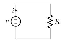
*Electric current — placed from the Real G.E.N.E.R.A.T.I.V.E. course library (Electronics room). Source: Wikimedia Commons (via Wikipedia article media). [Details & license](https://commons.wikimedia.org/wiki/File:Ohm%27s_Law_with_Voltage_source_TeX.svg).*

*Animated: Electric current — placed from the Real G.E.N.E.R.A.T.I.V.E. course library (Electronics room). Source: Wikimedia Commons (via Wikipedia article media). [Details & license](https://commons.wikimedia.org/wiki/File:Electromagnetic_induction_-_solenoid_to_loop_-_animation.gif).*
> An electric current is a flow of charged particles, such as electrons or ions, moving through an electrical conductor or space. It is defined as the net rate of flow of electric charge through a surface.[1]: 2 [2]: 622 The moving particles are called charge carriers, which may be one of several types of particles, depending on the conductor. ([Wikipedia](https://en.wikipedia.org/wiki/Electric_current))
<!-- REAL-GENERATIVE-MEDIA:END -->
<!-- SIGN-SYSTEMS:START -->
**Semiotic universals** (the notations and alphabet letters this article speaks — each opens its canonical card): flow · probability · temperature heat · emergence · exponential. Index: the glyph gallery · SEMIOTICS PORTAL.
<!-- SIGN-SYSTEMS:END -->
## Media (PD/CC)
<!-- MEDIA-DEPLOY:Electric_current/Electromagnetic_induction_-_solenoid_to_loop_-_animation.gif -->
!Gif Library/Electric current/Electromagnetic induction - solenoid to loop - animation.gif
*Electromagnetic_induction_-_solenoid_to_loop_-_animation.gif · Ponor · CC BY-SA 4.0 · [source](https://commons.wikimedia.org/wiki/File:Electromagnetic_induction_-_solenoid_to_loop_-_animation.gif)*
<!-- /MEDIA-DEPLOY -->
*SPINTRONICS · branch **P — Power transmission** · MicroSim pattern **J** (particles / agents): a sea of charge carriers drifting through a conductor. Draft staged by the headless draft queue; the publish stage adds frontmatter, the live editor iframe, and routes this into the Power-transmission branch folder.*
## Overview
**Electric current** is the rate at which electric charge flows past a point in a circuit. Its defining equation is simply
```
I = dQ / dt
```
— the charge `Q` (coulombs) crossing a cross-section per unit time `t` (seconds). The SI unit is the **ampere** (A): one ampere is one coulomb per second (`1 A = 1 C/s`). By the long-standing convention fixed before the [[Electron|electron]] was discovered, the **conventional current** points in the direction that *positive* charge would move; in an ordinary metal the actual carriers are electrons, so they drift the *opposite* way while the current is still drawn pointing "with the field."
Behind that macroscopic definition is a microscopic picture: a conductor holds an enormous reservoir of nearly-free charge carriers (about `8.5x10^28` electrons per cubic metre in [[Copper|copper]]) in ceaseless, fast, *random* thermal motion. Applying a field gives that random swarm a tiny **net drift**, and the current is the bookkeeping of that drift across the wire's cross-section:
```
I = n * q * v_d * A
```
The surprise the sketch is built around: the drift [[Velocity|velocity]] `v_d` is astonishingly small — fractions of a millimetre per second — even while the random thermal (Fermi) speed is around `10^6 m/s`. The current and its [[Energy|energy]] nonetheless appear almost instantly, because the *field* that nudges every carrier is established down the wire at nearly light speed; the carriers themselves barely crawl.
## The physics / derivation
**Current as flow of charge.** Mark a cross-section of area `A`. In a time `dt`, every carrier within a drift-distance `v_d*dt` of the plane crosses it. The volume swept is `A*v_d*dt`, it holds `n*A*v_d*dt` carriers each of charge `q`, so the charge crossing is `dQ = n*q*v_d*A*dt` and
```
I = dQ/dt = n * q * v_d * A
```
with `n` the carrier number [[Density|density]] (m^-3), `q` the charge per carrier (`e = 1.602x10^-19 C`), `v_d` the drift velocity (m/s), and `A` the cross-sectional area (m^2).
**Current density.** Dividing out the area gives the local, [[Geometry|geometry]]-free quantity
```
J = I / A = n * q * v_d (A/m^2)
```
**Drift from the field (Drude model).** Between collisions, a carrier of mass `m` is accelerated by the [[Force|force]] `qE`; averaged over the mean free time `tau`, it acquires a steady drift
```
v_d = (q*tau/m) * E = mu * E
```
where `mu = q*tau/m` is the **mobility** (m^2/V/s). Substituting back,
```
J = n*q*mu * E = sigma * E (microscopic Ohm's law)
```
so the **conductivity** is `sigma = n*q*mu` and the **resistivity** is `rho = 1/sigma`.
**Back to the macroscopic Ohm's law.** For a wire of length `L`, the field is `E = V/L` and the cross-section is `A`. Then
```
I = sigma*E*A = (sigma*A/L) * V = V / R, with R = rho*L/A = L/(sigma*A)
```
— the familiar `V = I*R` falls straight out of the drifting-swarm picture, with the resistance fixed by the material (`rho`) and the geometry (`L`, `A`).
**Why drift is so slow.** Solving `I = n*q*v_d*A` for a 1 A current in a 1 mm^2 copper wire gives `v_d = I/(n*q*A) ~ 7x10^-5 m/s` — about 0.07 mm/s, so a carrier takes hours to traverse a metre. The thermal/Fermi speed of those same electrons is `~1.6x10^6 m/s`, a ratio near `10^10`. The drift is a whisper-thin bias on a roaring random motion.
## Parameter table (controls -> real symbols)
| Control | Symbol | Meaning | Range (sim) |
|---------|:------:|---------|-------------|
| potential difference | `V` | [[Voltage|voltage]] across the `L = 0.10 m` segment; sets `E = V/L` | 0 – 25 mV |
| cross-sectional area | `A` | conductor cross-section; scales `I = J*A` | 0.5 – 10 mm^2 |
| material | `n, rho` | carrier density and resistivity: Copper / Aluminium / Nichrome | toggle |
*Fixed:* segment length `L = 0.10 m`, carrier charge `q = e`. *Derived and displayed:* field `E = V/L`, mobility `mu = 1/(n*q*rho)`, drift velocity `v_d = mu*E`, current density `J = sigma*E`, current `I = n*q*v_d*A = V/R`, resistance `R = rho*L/A`, the random Fermi speed `v_F` (for contrast), and a running charge odometer `Q = I*t` confirming `I = Q/t`.
## Learning objective
Understand that **electric current is the net drift of a carrier swarm**: `I = n*q*v_d*A`, that this is the same `I = dQ/dt` measured by counting charge through a cross-section, and that combining the microscopic Ohm's law `J = sigma*E` with the wire's geometry reproduces `V = I*R`. Above all, see the signature fact — the drift velocity `v_d` is minute (sub-mm/s) compared with the random thermal speed (`~10^6 m/s`), yet a large, steady current still flows.
<!-- CRAFT-LINK:START g12 -->
*Built to the [[WT!P5_js_Microsim_Master_Class|p5.js Master Class]].*
<!-- CRAFT-LINK:END -->
## Wikipedia : Wikitube
**Strict pair:** [Wikipedia](https://en.wikipedia.org/wiki/Electric_current) : [Wikitube](https://en.wikitube.io/wiki/Electric_current)
## Previous hub tags
Tree parents: [[Graph_theory]] · [[Reliability_engineering]].
Legacy hubs: none.
---
*Sources: 1 legacy note. Minted wave 1, 2026-07-30 (v1.6 order).*