# Magnetic resonance imaging
<!-- MICROSIMGEN:BEGIN v1.7 — generated by g08_place_microsims.py; three.js first (§15); do not hand-edit inside -->
## Microsims — p5.js
### Magnetic resonance imaging (p5.js) · `MRI`
<div class="microsim-player">
<iframe src="https://editor.p5js.org/sciencenibber/full/RjqYR__Lt" width="100%" height="480" frameborder="0" loading="lazy" sandbox="allow-scripts allow-same-origin" title="Magnetic resonance imaging — p5.js microsim"></iframe>
</div>
*Image soft tissue from the radio signals precessing nuclei emit in a strong field — Fourier reconstruction of the body.*
**Open in the editor:** [▶ fork this sketch](https://editor.p5js.org/sciencenibber/sketches/RjqYR__Lt) · movement *VIII · Imaging, audio & sensors* · library `p5js`
### Related microsims
Live sims on neighbouring articles — 1 of them inside this article's own Wikipedia link tree:
- [[Signal-to-noise_ratio]] *(in tree)*
- [[Decibel]]
- [[Digital_image_processing]]
- [[Distortion]]
- [[Sensor]]
- [[Transducer]]
*Sim hosted off-article; the article owns the reference, not the runtime (WIKI_RULES §10.4). Placed by `g08_place_microsims.py`.*
<!-- g09-shelf-note -->
> **Also on this page:** 1 further p5.js sketch already published for this article live further down. Per WIKI_RULES §5 a collision promotes rather than forks — they are one shelf, not rivals; this block is the §10.4 *current best* reference.
<!-- MICROSIMGEN:END -->
## Microsim
### Live player
<div class="microsim-player">
<iframe src="https://editor.p5js.org/sciencenibber/full/NXAxGfamM" width="100%" height="620" frameborder="0" sandbox="allow-scripts allow-same-origin"></iframe>
</div>
<div class="microsim-fallback">
<img src="Microsims/thumbs/Magnetic_resonance_imaging.png" alt="Magnetic_resonance_imaging microsim poster" style="width:100%;border:1px solid #4445;border-radius:6px;">
<p><em>Live microsim (desktop) · <a href="https://editor.p5js.org/sciencenibber/sketches/NXAxGfamM">open sketch in the p5.js editor</a></em></p>
</div>
**Editor URL:** https://editor.p5js.org/sciencenibber/sketches/NXAxGfamM
**Description (100 words):**
A nine-[[Block_diagram|block diagram]] of the MRI signal chain — cryostat, NbTi [[Superconducting_magnet|superconducting magnet]], shim and gradient coils, RF transmit, the patient and its protons, RF receive, preamp/ADC, k-space buffer, and 2D FFT — wired together with coloured arrows. Coloured tokens flow along the arrows on every TR boundary, k-space fills row by row in centric order, and the reconstructed image emerges in a small preview pane on the right. Sliders set the main field (B_0, 0.5–7 T) and repetition time (TR); buttons switch between SE, GRE, and EPI sequences. The Larmor frequency readout updates live with B_0.
```js
// =====================================================================
// Magnetic_resonance_imaging.js -- Wikitube microsim
// Article: Magnetic_resonance_imaging
// URL: en.wikitube.io/wiki/Magnetic_resonance_imaging
// Room: Helium Pattern: G (block diagrams, system flows)
// ---------------------------------------------------------------------
// Idea: an interactive block diagram of the MRI signal chain, from the
// cryostat that holds liquid helium at 4.2 K all the way to the
// reconstructed image. The reader scrubs B0 (field strength), TR
// (repetition time) and the pulse-sequence selector, then watches
// animated tokens flow through the chain while k-space fills row by
// row and the image emerges from the inverse 2D Fourier transform.
//
// Block layout (9 stations, 3 rows of 3):
//
// row 1 -- B0 magnetic system (helium-dependent half of the scanner)
// [Cryostat 4.2 K] -> [NbTi Magnet B_0] -> [Shim & Gradient coils]
// |
// v
// row 2 -- RF excitation and reception (around the patient)
// [RF Transmit B_1] ----> [Patient / Spins] ----> [RF Receive coil]
// |
// v
// row 3 -- digital signal chain (back-end of the scanner)
// [Preamp + ADC] ----> [k-space buffer] ----> [2D FFT -> Image]
//
// The top row is the structural reason this article lives in the
// Helium room: every clinical 1.5T / 3T / 7T magnet is a NbTi
// superconducting solenoid sitting in a 2000-litre liquid-helium
// bath at 4.222 K. No He-4, no MRI -- which is why helium policy is
// upstream of every radiology department in the country.
//
// Canonical equations driven by the controls:
//
// omega_0 = gamma * B_0 (Larmor precession)
// gamma/(2*pi) = 42.58 MHz/T for 1H
//
// M_z(t) = M_0 * (1 - exp(-t/T1)) (longitudinal recovery)
// M_xy(t) = M_0 * exp(-t/T2) (transverse decay)
//
// I(x, y) = inverse_2D_FFT[ S(kx, ky) ] (image reconstruction)
//
// Controls:
// * B_0 slider (0.5 - 7.0 T) -- updates the Larmor frequency
// readout in real time
// * TR slider (10 - 500 ms) -- repetition time; faster TR =>
// faster k-space fill rate
// * 3 sequence buttons (SE / GRE / EPI) -- changes the token color
// and the per-TR k-space lines
// (EPI fills 4 lines per TR, SE
// and GRE fill 1)
// * "reset image" button -- clears k-space and starts over
//
// Visual layout (720 x 520 canvas):
// * y 0 - 50 HUD: title, URL, control hints (top-right)
// * y 55 - 320 block diagram with animated tokens on arrows
// * y 325 - 395 controls: 2 sliders, 3 sequence buttons, reset
// * y 400 - 480 three preview panes:
// (a) k-space magnitude (32x32, fills as scan
// progresses)
// (b) phase-encode "line" gauge
// (c) reconstructed image (32x32, revealed as
// more k-space lines accumulate)
// * y 485 - 515 bottom strip: live readouts + canonical equation
//
// Conventions (Wikitube Betterfire Standard v0, P5_JS_EDITOR section 2):
// * single ARTICLE constant, single quotes
// * p5.disableFriendlyErrors = true to keep the editor console clean
// * non-ASCII characters (omega, gamma, lambda, arrows) ONLY appear
// in comments; every text() call uses pure ASCII so the editor
// preview pipeline doesn't mangle them
// * Energy room palette from P5_JS_EDITOR section 4 line 165:
// BG=18, FG=240, HOT=[220,110,60], COLD=[60,130,220],
// STRUCT=[120,130,150], TRAJ=[240,220,80]
//
// Pre-fab "phantom" image: an axial-slice-flavoured shape (oval head
// outline + two ventricle disks + a small lesion). The point is to
// reveal a recognisable thing as k-space fills, not to be a medically
// faithful reconstruction.
// =====================================================================
const ARTICLE = 'Magnetic_resonance_imaging';
const TITLE = ARTICLE.replace(/_/g, ' ');
p5.disableFriendlyErrors = true;
// ----- Energy room palette (P5_JS_EDITOR section 4, line 165) --------
const BG = 18;
const FG = 240;
const DIM = [240, 240, 240, 140];
const HOT = [220, 110, 60]; // RF (B_1) excitation, "warm" half
const COLD = [60, 130, 220]; // B_0 field, cryogenic half
const COLDER = [40, 80, 180]; // deeper cool for liquid-He block
const STRUCT = [120, 130, 150]; // outlines, neutral structure
const TRAJ = [240, 220, 80]; // echo / signal accent
const ACCENT = [200, 100, 220]; // k-space accent (magenta)
const GAUGE = [120, 220, 140]; // image-progress gauge
// ----- Physics constants ---------------------------------------------
// gamma/(2*pi) for the 1H proton, in MHz per Tesla.
const GAMMA_OVER_2PI_MHZ_PER_T = 42.577;
// Phantom image size and k-space size. Square, power-of-two-friendly.
const N_K = 32;
// Per-sequence "lines per TR" -- how many k-space rows are written in
// one TR period. EPI is the speed king of clinical sequences because
// it reads many lines per excitation.
const LINES_PER_TR = { SE: 1, GRE: 1, EPI: 4 };
// ----- Block-diagram graph -------------------------------------------
// 9 blocks in 3 rows of 3. The arrows form a serpentine: row 1 LTR,
// down on the right, row 2 LTR (with the patient as the hub), down on
// the right again, row 3 LTR. Plus extra arrows from row 1's gradient
// block down to the patient, and a top-down B_0 arrow from the magnet
// to the patient -- those carry "field" tokens.
const BLOCK_W = 170;
const BLOCK_H = 56;
const BLOCK_GAP_X = 30;
// Row Y centres (set in setup once canvas is known).
let blocks = []; // { id, label, sub, x, y, w, h, group }
let edges = []; // { from, to, route: [ {x,y}, ... ], group, baseRate }
// ----- Animated tokens -----------------------------------------------
// Each token rides one edge with a parametric u in [0, 1]. Color and
// label come from the token's "kind" (B0 field, B1 pulse, echo, data).
let tokens = []; // { edgeIdx, u, kind, color, speed }
// ----- Scanner state -------------------------------------------------
let B0 = 1.5; // Tesla
let TR = 60; // ms (slider-driven)
let seq = 'SE'; // sequence key, default Spin Echo
let kRow = 0; // next k-space row to fill (0..N_K-1)
let kFilled = 0; // count of rows filled (0..N_K), for progress gauge
let trClock = 0; // ms accumulator within the current TR window
// Buffers for the previews.
let kMag = []; // 2D array N_K x N_K, magnitude of complex k-space
let imageBuf = []; // 2D array N_K x N_K, reconstructed image (greyscale)
let phantom = []; // 2D array N_K x N_K, the "true" image (oval head)
// Sliders and buttons (UI handles).
let b0Slider, trSlider;
let btnSE, btnGRE, btnEPI, btnReset;
// Pre-rendered phantom Fourier magnitude (so we don't re-FFT each row).
let phantomFourier = []; // N_K x N_K magnitudes
function setup() {
createCanvas(720, 520);
pixelDensity(2);
textFont('system-ui');
// ---- Build the block-diagram graph -------------------------------
// Row y centres inside the diagram band (y = 55 .. 320, three rows).
const rowY = [110, 195, 280];
const xCol = [60, 60 + BLOCK_W + BLOCK_GAP_X, 60 + 2 * (BLOCK_W + BLOCK_GAP_X)];
blocks = [
// Row 1 -- helium-cooled magnetic system
{ id: 'cryo', label: 'Cryostat', sub: 'liquid He, 4.2 K',
x: xCol[0], y: rowY[0], w: BLOCK_W, h: BLOCK_H, group: 'cryo' },
{ id: 'magn', label: 'NbTi Magnet', sub: 'B_0 main field',
x: xCol[1], y: rowY[0], w: BLOCK_W, h: BLOCK_H, group: 'cryo' },
{ id: 'grad', label: 'Shim & Gradients', sub: 'G_x, G_y, G_z',
x: xCol[2], y: rowY[0], w: BLOCK_W, h: BLOCK_H, group: 'cryo' },
// Row 2 -- RF excitation, the patient, RF reception
{ id: 'rftx', label: 'RF Transmit', sub: 'B_1 at omega_0',
x: xCol[0], y: rowY[1], w: BLOCK_W, h: BLOCK_H, group: 'rf' },
{ id: 'patient', label: 'Patient / Spins', sub: '1H protons in tissue',
x: xCol[1], y: rowY[1], w: BLOCK_W, h: BLOCK_H, group: 'sample' },
{ id: 'rfrx', label: 'RF Receive', sub: 'tuned coil',
x: xCol[2], y: rowY[1], w: BLOCK_W, h: BLOCK_H, group: 'echo' },
// Row 3 -- digital signal chain
{ id: 'adc', label: 'Preamp + ADC', sub: 'I / Q demod',
x: xCol[0], y: rowY[2], w: BLOCK_W, h: BLOCK_H, group: 'data' },
{ id: 'kspace', label: 'k-space buffer', sub: 'S(k_x, k_y)',
x: xCol[1], y: rowY[2], w: BLOCK_W, h: BLOCK_H, group: 'data' },
{ id: 'fft', label: '2D FFT -> Image', sub: 'I(x, y)',
x: xCol[2], y: rowY[2], w: BLOCK_W, h: BLOCK_H, group: 'image' }
];
// ---- Edges (arrows) ----------------------------------------------
// Each edge has a route: a polyline in canvas pixels along which a
// token rides parametrically. Horizontal arrows go centre-to-centre
// at the row's y. Vertical drops use the right-edge of the source
// block down to the left-edge of the next row.
function blk(id) { return blocks.find(b => b.id === id); }
function rightMid(b) { return { x: b.x + b.w, y: b.y + b.h / 2 }; }
function leftMid(b) { return { x: b.x, y: b.y + b.h / 2 }; }
function bottomMid(b) { return { x: b.x + b.w / 2, y: b.y + b.h }; }
function topMid(b) { return { x: b.x + b.w / 2, y: b.y }; }
edges = [
// Row 1 horizontal: cryo -> magn -> grad
{ from: 'cryo', to: 'magn', group: 'cryo',
route: [ rightMid(blk('cryo')), leftMid(blk('magn')) ], baseRate: 0.4 },
{ from: 'magn', to: 'grad', group: 'cryo',
route: [ rightMid(blk('magn')), leftMid(blk('grad')) ], baseRate: 0.4 },
// Magnet -> patient (steady B_0 field flowing down)
{ from: 'magn', to: 'patient', group: 'B0',
route: [ bottomMid(blk('magn')), topMid(blk('patient')) ], baseRate: 0.25 },
// Gradients -> patient (G(t) carries spatial encoding to the spins)
{ from: 'grad', to: 'patient', group: 'grad',
route: [
bottomMid(blk('grad')),
{ x: blk('grad').x + blk('grad').w / 2, y: rowY[1] - 18 },
{ x: blk('patient').x + blk('patient').w / 2 + 30, y: rowY[1] - 18 },
{ x: blk('patient').x + blk('patient').w / 2 + 30,
y: blk('patient').y } ], baseRate: 0.55 },
// RF Tx -> patient (excitation pulse, the "warm" half)
{ from: 'rftx', to: 'patient', group: 'rf',
route: [ rightMid(blk('rftx')), leftMid(blk('patient')) ], baseRate: 0.9 },
// Patient -> RF Rx (the spin echo flying out of the sample)
{ from: 'patient', to: 'rfrx', group: 'echo',
route: [ rightMid(blk('patient')), leftMid(blk('rfrx')) ], baseRate: 0.9 },
// RF Rx -> ADC: drop down one row then over to the preamp
{ from: 'rfrx', to: 'adc', group: 'echo',
route: [
bottomMid(blk('rfrx')),
{ x: blk('rfrx').x + blk('rfrx').w / 2, y: rowY[2] - 30 },
{ x: blk('adc').x + blk('adc').w / 2, y: rowY[2] - 30 },
topMid(blk('adc'))
], baseRate: 0.7 },
// Row 3 horizontal: ADC -> k-space -> FFT
{ from: 'adc', to: 'kspace', group: 'data',
route: [ rightMid(blk('adc')), leftMid(blk('kspace')) ], baseRate: 0.7 },
{ from: 'kspace', to: 'fft', group: 'data',
route: [ rightMid(blk('kspace')), leftMid(blk('fft')) ], baseRate: 0.6 }
];
// ---- Phantom and its Fourier magnitudes --------------------------
buildPhantom();
buildPhantomFourier();
// ---- Initialise k-space and image buffers ------------------------
resetScanState();
// ---- Sliders and buttons -----------------------------------------
// Layout band: y = 325 .. 395
const ctrlY = 332;
b0Slider = createSlider(0.5, 7.0, 1.5, 0.1).position(20, ctrlY).size(190);
trSlider = createSlider(10, 500, 60, 5).position(20, ctrlY + 28).size(190);
btnSE = createButton('SE'); btnSE.position(240, ctrlY + 24).size(50, 24);
btnGRE = createButton('GRE'); btnGRE.position(296, ctrlY + 24).size(54, 24);
btnEPI = createButton('EPI'); btnEPI.position(356, ctrlY + 24).size(50, 24);
btnSE .mousePressed (() => { seq = 'SE'; });
btnGRE.mousePressed (() => { seq = 'GRE'; });
btnEPI.mousePressed (() => { seq = 'EPI'; });
btnReset = createButton('reset image');
btnReset.position(420, ctrlY + 24).size(110, 24);
btnReset.mousePressed(() => { resetScanState(); });
// ---- Seed a couple of steady "field" tokens on the cryo row ------
tokens.push({ edgeIdx: 0, u: 0.0, kind: 'cryo', color: COLDER, speed: 0.15 });
tokens.push({ edgeIdx: 1, u: 0.0, kind: 'B0', color: COLD, speed: 0.15 });
tokens.push({ edgeIdx: 2, u: 0.0, kind: 'B0', color: COLD, speed: 0.12 });
}
// =====================================================================
// Phantom image -- a soft oval "head" with two darker disks for
// ventricles and a tiny bright lesion. Pre-baked once.
// =====================================================================
function buildPhantom() {
phantom = [];
for (let j = 0; j < N_K; j++) {
phantom.push([]);
for (let i = 0; i < N_K; i++) {
const x = (i - N_K / 2 + 0.5) / (N_K / 2); // -1 .. 1
const y = (j - N_K / 2 + 0.5) / (N_K / 2);
// Ellipse: (x/0.65)^2 + (y/0.9)^2 < 1
const inHead = (x / 0.65) * (x / 0.65) + (y / 0.9) * (y / 0.9) < 1;
// Two ventricles (small circles)
const d1 = Math.hypot(x + 0.18, y - 0.05);
const d2 = Math.hypot(x - 0.18, y - 0.05);
// Lesion (tiny bright spot in lower-right of head)
const dL = Math.hypot(x - 0.25, y + 0.30);
let v = 0;
if (inHead) {
v = 0.55; // grey-matter base
if (d1 < 0.13) v = 0.20; // left ventricle (dark)
if (d2 < 0.13) v = 0.20; // right ventricle
if (dL < 0.06) v = 1.00; // bright lesion
// Smooth skull rim
const rEdge = Math.sqrt((x / 0.65) ** 2 + (y / 0.9) ** 2);
if (rEdge > 0.93) v *= map(rEdge, 0.93, 1.0, 1.0, 0.0);
}
phantom[j].push(v);
}
}
}
// Build the magnitude of the 2D DFT of the phantom. Used as the
// content that fills k-space, one row at a time. We compute a full
// DFT here -- N_K = 32 so it's only 1024 cells x 1024 sample sums =
// 1M ops, one-time at setup, well within budget.
function buildPhantomFourier() {
phantomFourier = [];
for (let v = 0; v < N_K; v++) {
phantomFourier.push([]);
for (let u = 0; u < N_K; u++) {
let re = 0, im = 0;
for (let j = 0; j < N_K; j++) {
for (let i = 0; i < N_K; i++) {
const p = phantom[j][i];
if (p === 0) continue;
const ang = -2 * Math.PI * (u * i / N_K + v * j / N_K);
re += p * Math.cos(ang);
im += p * Math.sin(ang);
}
}
phantomFourier[v].push(Math.hypot(re, im));
}
}
}
// =====================================================================
// Reconstruction. To keep frame budget small, we don't re-IFFT every
// frame. Instead, the reconstructed image at each step is just the
// phantom partially masked by the fraction of k-space rows filled --
// which is what the eye reads as "k-space lines accumulate into a
// recognisable image". This is a teaching simplification, not the
// real thing; the real reconstruction is the inverse 2D FFT.
// =====================================================================
function reconstructPartial() {
imageBuf = [];
const frac = kFilled / N_K; // 0 .. 1
for (let j = 0; j < N_K; j++) {
imageBuf.push([]);
for (let i = 0; i < N_K; i++) {
// Blurry partial reconstruction:
// blend phantom with mean grey by fraction filled, and add
// a touch of streaking noise at low fill (Gibbs-flavoured).
const m = phantom[j][i];
let noise = 0;
if (frac < 1.0) {
// small horizontal streaks if the missing rows are k-y > kFilled
noise = (random() - 0.5) * (1 - frac) * 0.18;
}
const v = m * (0.35 + 0.65 * frac) + noise;
imageBuf[j].push(constrain(v, 0, 1));
}
}
}
function resetScanState() {
kFilled = 0;
kRow = 0;
trClock = 0;
kMag = [];
for (let j = 0; j < N_K; j++) {
kMag.push(new Array(N_K).fill(0));
}
reconstructPartial();
}
// =====================================================================
// Per-frame update: advance TR clock, fill k-space rows on each TR
// boundary, advance tokens along their edges.
// =====================================================================
function update() {
// Read sliders once per frame.
B0 = b0Slider.value();
TR = trSlider.value();
// Real elapsed milliseconds since last frame. Capped to keep
// background-tab resumes from blowing up the scheduler.
const dt = Math.min(deltaTime, 100);
trClock += dt;
// On each TR boundary, fill `lines per TR` more rows of k-space and
// spawn one echo token down the chain. EPI fills 4 lines per TR.
while (trClock >= TR && kFilled < N_K) {
trClock -= TR;
const lines = LINES_PER_TR[seq];
for (let n = 0; n < lines && kFilled < N_K; n++) {
// Choose a row to fill -- "centric" order, alternating in and
// out from the centre, which is roughly how real EPI / spiral
// fills go. Pure linear fill is also fine; centric is prettier.
const j = kRowOrder(kFilled);
for (let i = 0; i < N_K; i++) {
kMag[j][i] = phantomFourier[j][i];
}
kFilled += 1;
kRow = (kRow + 1) % N_K;
}
// Spawn one excitation token through the RF Tx -> patient edge
spawnEchoChain();
}
// Update partial reconstruction (cheap; recomputed from a single
// multiplicative formula).
reconstructPartial();
// Advance every token along its edge.
for (const t of tokens) {
const rate = (edges[t.edgeIdx].baseRate) * (t.speed) * (dt / 1000);
t.u += rate;
}
// Loop "field" tokens (B0, cryo, grad) -- they cycle forever.
// Excitation / echo / data tokens are removed when they reach u=1.
tokens = tokens.filter(t => {
if (t.u < 1) return true;
if (t.kind === 'B0' || t.kind === 'cryo' || t.kind === 'grad') {
t.u = 0; // wrap
return true;
}
return false;
});
}
// Centric k-space row order: 16, 17, 15, 18, 14, 19, 13, ...
// Given the count `n` of rows filled so far (0..N_K-1), return the
// next row index.
function kRowOrder(n) {
const c = Math.floor(N_K / 2);
if (n === 0) return c;
const half = Math.ceil(n / 2);
return n % 2 === 1 ? c + half : c - half;
}
// One "shot" of the pulse sequence: a B1 excitation token travels
// from RF Tx into the patient, then an echo token travels from the
// patient out to RF Rx and on through the digital chain.
function spawnEchoChain() {
// RF Tx -> patient (B1 pulse, hot orange)
tokens.push({ edgeIdx: edgeIndex('rftx', 'patient'),
u: 0, kind: 'B1', color: HOT, speed: 1.6 });
// Patient -> RF Rx (echo, traj yellow), short delay implied by
// starting it at u = -0.3 (we let the update pass clamp it).
tokens.push({ edgeIdx: edgeIndex('patient', 'rfrx'),
u: -0.25, kind: 'echo', color: TRAJ, speed: 1.4 });
// RF Rx -> ADC -> kspace -> FFT
tokens.push({ edgeIdx: edgeIndex('rfrx', 'adc'),
u: -0.6, kind: 'data', color: GAUGE, speed: 1.0 });
tokens.push({ edgeIdx: edgeIndex('adc', 'kspace'),
u: -1.0, kind: 'data', color: GAUGE, speed: 0.9 });
tokens.push({ edgeIdx: edgeIndex('kspace', 'fft'),
u: -1.4, kind: 'data', color: ACCENT, speed: 0.8 });
}
function edgeIndex(fromId, toId) {
for (let i = 0; i < edges.length; i++) {
if (edges[i].from === fromId && edges[i].to === toId) return i;
}
return 0;
}
// =====================================================================
// Rendering
// =====================================================================
function draw() {
background(BG);
update();
// ---- Block diagram ----------------------------------------------
drawEdges();
drawTokens();
drawBlocks();
// ---- Control labels ---------------------------------------------
drawControlLabels();
// ---- Preview panes (k-space + progress + image) ------------------
drawKspacePreview(20, 410, 70);
drawProgressGauge(110, 410, 70);
drawImagePreview(630, 410, 70);
// ---- Bottom readouts + canonical equation ------------------------
drawReadouts();
// ---- HUD (top, painted last so it sits on top) -------------------
drawHUD();
}
function drawBlocks() {
noStroke();
for (const b of blocks) {
// Background tint by group
const tint = groupTint(b.group);
fill(tint[0], tint[1], tint[2], 40);
rect(b.x, b.y, b.w, b.h, 6);
// Outline
stroke(...STRUCT);
strokeWeight(1);
noFill();
rect(b.x, b.y, b.w, b.h, 6);
// Label
noStroke();
fill(FG);
textAlign(CENTER, CENTER);
textSize(13);
text(b.label, b.x + b.w / 2, b.y + 18);
fill(...DIM);
textSize(10);
text(b.sub, b.x + b.w / 2, b.y + 38);
}
}
function drawEdges() {
for (const e of edges) {
stroke(...edgeColor(e.group));
strokeWeight(1.4);
noFill();
beginShape();
for (const pt of e.route) vertex(pt.x, pt.y);
endShape();
// Arrow head at the last segment
const a = e.route[e.route.length - 2];
const b = e.route[e.route.length - 1];
drawArrowHead(a, b, edgeColor(e.group));
}
}
function drawArrowHead(a, b, col) {
const ang = Math.atan2(b.y - a.y, b.x - a.x);
const s = 7;
push();
translate(b.x, b.y);
rotate(ang);
noStroke();
fill(...col);
triangle(0, 0, -s, -s * 0.55, -s, s * 0.55);
pop();
}
function drawTokens() {
noStroke();
for (const t of tokens) {
if (t.u < 0) continue;
const pos = sampleRoute(edges[t.edgeIdx].route, constrain(t.u, 0, 1));
fill(...t.color);
circle(pos.x, pos.y, t.kind === 'B0' || t.kind === 'cryo' ? 5 : 7);
}
}
// Sample a polyline at parametric u in [0,1] by arc length.
function sampleRoute(route, u) {
if (route.length < 2) return route[0];
// Total length
let total = 0;
const segLens = [];
for (let i = 0; i < route.length - 1; i++) {
const dx = route[i + 1].x - route[i].x;
const dy = route[i + 1].y - route[i].y;
const L = Math.hypot(dx, dy);
segLens.push(L);
total += L;
}
let target = u * total;
for (let i = 0; i < segLens.length; i++) {
if (target <= segLens[i]) {
const f = segLens[i] === 0 ? 0 : target / segLens[i];
return {
x: lerp(route[i].x, route[i + 1].x, f),
y: lerp(route[i].y, route[i + 1].y, f)
};
}
target -= segLens[i];
}
return route[route.length - 1];
}
// Map a block's "group" to its background tint colour.
function groupTint(g) {
if (g === 'cryo') return COLDER;
if (g === 'rf') return HOT;
if (g === 'sample') return STRUCT;
if (g === 'echo') return TRAJ;
if (g === 'data') return GAUGE;
if (g === 'image') return ACCENT;
return STRUCT;
}
// Map an edge group to its line colour.
function edgeColor(g) {
if (g === 'cryo') return COLDER;
if (g === 'B0') return COLD;
if (g === 'grad') return [180, 180, 220];
if (g === 'rf') return HOT;
if (g === 'echo') return TRAJ;
if (g === 'data') return GAUGE;
return STRUCT;
}
// =====================================================================
// Preview panes
// =====================================================================
function drawKspacePreview(x0, y0, size) {
push();
noStroke();
fill(...DIM);
textSize(10);
textAlign(LEFT, BOTTOM);
text('k-space S(k_x, k_y)', x0, y0 - 4);
// Find a max for normalisation
let mx = 1e-6;
for (let j = 0; j < N_K; j++) {
for (let i = 0; i < N_K; i++) {
if (kMag[j][i] > mx) mx = kMag[j][i];
}
}
// Log compression for visual punch (k-space magnitude is heavy-tailed)
const cell = size / N_K;
for (let j = 0; j < N_K; j++) {
for (let i = 0; i < N_K; i++) {
const m = kMag[j][i] / mx;
const v = m > 0 ? 255 * Math.pow(m, 0.35) : 0;
fill(v, v * 0.75, v * 0.45);
rect(x0 + i * cell, y0 + j * cell, cell + 1, cell + 1);
}
}
// Frame
noFill();
stroke(...STRUCT);
strokeWeight(1);
rect(x0, y0, size, size);
pop();
}
function drawProgressGauge(x0, y0, size) {
push();
noStroke();
fill(...DIM);
textSize(10);
textAlign(LEFT, BOTTOM);
text('phase-encode lines', x0, y0 - 4);
// Vertical stack of N_K thin bars, lit up to kFilled in centric order.
const cellH = size / N_K;
// Pre-compute order so we can light the actual order, not 0..kFilled.
const order = [];
for (let n = 0; n < N_K; n++) order.push(kRowOrder(n));
for (let j = 0; j < N_K; j++) {
const isFilled = order.slice(0, kFilled).indexOf(j) >= 0;
fill(...(isFilled ? TRAJ : [60, 60, 80]));
rect(x0, y0 + j * cellH, size, cellH - 0.5);
}
// Border
noFill();
stroke(...STRUCT);
strokeWeight(1);
rect(x0, y0, size, size);
// Centred caption: NN / 32
noStroke();
fill(FG);
textSize(11);
textAlign(CENTER, CENTER);
text(kFilled + ' / ' + N_K, x0 + size / 2, y0 + size + 14);
pop();
}
function drawImagePreview(xRight, y0, size) {
// Drawn right-aligned: x0 = xRight - size
const x0 = xRight - size;
push();
noStroke();
fill(...DIM);
textSize(10);
textAlign(RIGHT, BOTTOM);
text('reconstructed image I(x, y)', xRight, y0 - 4);
const cell = size / N_K;
for (let j = 0; j < N_K; j++) {
for (let i = 0; i < N_K; i++) {
const v = imageBuf[j][i];
const g = 255 * v;
fill(g, g, g);
rect(x0 + i * cell, y0 + j * cell, cell + 1, cell + 1);
}
}
// Frame
noFill();
stroke(...STRUCT);
strokeWeight(1);
rect(x0, y0, size, size);
pop();
}
// =====================================================================
// Control labels (sliders are DOM, so we draw their captions on canvas)
// =====================================================================
function drawControlLabels() {
push();
noStroke();
fill(...DIM);
textAlign(LEFT, BOTTOM);
textSize(11);
text('B_0 main field = ' + B0.toFixed(1) + ' T', 20, 332);
text('TR repetition time = ' + TR + ' ms', 20, 360);
textAlign(LEFT, CENTER);
textSize(11);
fill(...DIM);
text('pulse sequence', 240, 348);
// Highlight the active sequence button by drawing a halo behind it.
const xs = { SE: 240, GRE: 296, EPI: 356 };
const ws = { SE: 50, GRE: 54, EPI: 50 };
const ax = xs[seq], aw = ws[seq];
noFill();
stroke(...HOT);
strokeWeight(2);
rect(ax - 2, 354, aw + 4, 28, 4);
pop();
}
// =====================================================================
// Bottom readouts + canonical equation
// =====================================================================
function drawReadouts() {
push();
// Larmor frequency: omega_0 / (2*pi) = gamma/(2*pi) * B_0, in MHz
const fLarmorMHz = GAMMA_OVER_2PI_MHZ_PER_T * B0;
noStroke();
fill(FG);
textAlign(LEFT, BOTTOM);
textSize(12);
const line1 =
'B_0 = ' + B0.toFixed(1) + ' T ' +
'Larmor freq = ' + fLarmorMHz.toFixed(2) + ' MHz ' +
'seq = ' + seq + ' ' +
'TR = ' + TR + ' ms';
text(line1, 14, height - 22);
// Canonical equation (Betterfire Standard rule 4) -- bottom-right
textAlign(RIGHT, BOTTOM);
fill(FG);
textSize(13);
text('omega_0 = gamma * B_0 [Larmor precession]',
width - 14, height - 6);
// Bottom-left subtitle: progress + helium reminder
textAlign(LEFT, BOTTOM);
fill(...DIM);
textSize(11);
text('k-space ' + Math.round(100 * kFilled / N_K) + '% filled ' +
'| NbTi magnet bathed in liquid He at 4.2 K',
14, height - 6);
pop();
}
// =====================================================================
// HUD
// =====================================================================
function drawHUD() {
// Top-left: title + Wikitube URL (Betterfire Standard rules 1, 2)
noStroke();
fill(FG);
textAlign(LEFT, TOP);
textSize(22);
text(TITLE, 14, 10);
fill(...DIM);
textSize(12);
text('Wikitube microsim . en.wikitube.io/wiki/' + ARTICLE, 14, 38);
// Top-right: control hints (Betterfire Standard rule 3)
textAlign(RIGHT, TOP);
fill(...DIM);
textSize(10);
text('drag B_0 and TR sliders to retune', width - 14, 12);
text('SE / GRE / EPI buttons swap the sequence', width - 14, 24);
text('reset image to clear k-space', width - 14, 36);
}
// =====================================================================
// End of Magnetic_resonance_imaging.js
// Wikitube microsim, Helium room, Pattern G (block diagram).
// =====================================================================
```
## Links (Wikipedia order)
<!-- injected from _registry/childlinks/Magnetic_resonance_imaging.json (2026-07-30T02:09:12Z) -->
`Abbreviation` · `Abrikosov_vortex` · `Agence_France-Presse` · `Aliasing` · `Alzheimer's_disease` · `Anaphylaxis` · `Anatomy` · `Andreev_reflection` · `Aneurysm` · `Angiography` · `Arrhythmia` · `Artificial_intelligence_in_healthcare` · `Atomic_nucleus` · `Autopsy` · `BCS_theory` · `Bean's_critical_state_model` · `Bilayer_graphene` · `Bile_duct` · `Bloch_equations` · `Bone` · `Brainstem` · `Brownian_motion` · `CT_scan` · `Calcification` · `Cancer_staging` · `Carbon-13` · `Cardiomyopathy` · `Central_nervous_system` · `Cerebellum` · `Cerebrospinal_fluid` · `Chest_radiograph` · `Claustrophobia` · `Cochlear_implant` · `Colorectal_cancer` · `Composition_of_the_human_body` · `Compressed_sensing` · `Concentration` · `Confocal_microscopy` · `Congenital_heart_defect` · `Consumer_Reports` · `Contrast_(vision)` · `Contrast_agent` · `Conventional_superconductor` · `Cooper_pair` · `Coordination_sphere` · [[Copper]] · `Coronary_artery_disease` · `Covalent_superconductor` · `Critical_field` · `Cryotron` · `Cuprate_superconductor` · `Dementia` · `Demyelinating_disease` · `Deuterium` · `Diamagnetism` · `Diffuse_axonal_injury` · `Dual-energy_X-ray_absorptiometry` · `Echocardiography` · `Edema` · `Electron_paramagnetic_resonance` · `Epilepsy` · `Excited_state` · `Exogeny` · `Fat` · `Ferritin` · `Ferromagnetic_superconductor` · `Ferromagnetism` · `Fibrosis` · [[Fluorine]] · `Fluoroscopy` · `Flux_pinning` · `Flux_pumping` · `Focused_assessment_with_sonography_for_trauma` · `Food_and_Drug_Administration` · `Forensic_science` · `Fractional_anisotropy` · `Functional_magnetic_resonance_imaging` · `Gadodiamide` · [[Gadolinium]] · `Gallium_scan` · `Gamma_ray` · `Ginzburg–Landau_theory` · `Grey_matter` · `Gyromagnetic_ratio` · `Harvard_Medical_School` · `Health_system` · `Hearing_loss` · `Hearing_protection_device` · `Heart` · `Heavy_fermion_superconductor` · [[Helium-3]] · `Hemoglobin` · `Hemosiderin` · `High-resolution_computed_tomography` · `High-temperature_superconductivity` · `History_of_neuroimaging` · `Homes's_law` · `Homogeneity_(physics)` · [[Hydrogen]] · `Hyperacusis` · `Hyperfine_structure` · `Hyperpolarization_(physics)` · `ICD-9-CM_Volume_3` · `Infection` · `Inflammation` · `Integrated_circuit` · `Interventional_radiology` · `Intravenous_therapy` · `Ionizing_radiation` · [[Iron]] · `Iron-based_superconductor` · `Iron_overload` · `Iterative_reconstruction` · `J-coupling` · `Joint` · `Joint_injection` · `Josephson_effect` · `Kidney_dialysis` · `Kidney_failure` · `Kohn–Luttinger_superconductivity` · `Lanthanum_barium_copper_oxide` · `Larmor_precession` · `Laser` · [[Liquid_helium]] · `List_of_infections_of_the_central_nervous_system` · `List_of_superconductors` · `Little–Parks_effect` · `Liver` · `London_equations` · `London_penetration_depth` · `Low_back_pain` · `Lower_gastrointestinal_series` · `MRI_contrast_agent` · `Magnesium_diboride` · `Magnet` · `Magnetic_dipole` · `Magnetic_field` · `Magnetic_resonance_angiography` · `Magnetic_resonance_imaging_of_the_brain` · `Magnetization` · `Magnetostriction` · [[Manganese]] · `Massachusetts_General_Hospital` · `Matthias_rules` · `Mattis–Bardeen_theory` · `Medical_Subject_Headings` · `Medical_diagnosis` · `Medical_imaging` · `Medical_optical_imaging` · `Medical_ultrasound` · `MedlinePlus` · `Meissner_effect` · `Melanin` · `Meningitis` · `Metabolism` · `Molecular_imaging` · `Multiple_sclerosis` · `Myocardial_perfusion_imaging` · `Myocarditis` · `Nephrogenic_systemic_fibrosis` · `Neuroimaging` · `Niobium–tin` · `Niobium–titanium` · `Nobel_Prize_in_Physiology_or_Medicine` · [[Nuclear_magnetic_resonance]] · `Nuclear_magnetic_resonance_spectroscopy` · `Nuclear_medicine` · `OECD` · `Optical_coherence_tomography` · `Oral_administration` · `Orbit_(anatomy)` · `Organic_superconductor` · [[Oscillation]] · `Oxford_University_Press` · `Oxygen_saturation_(medicine)` · `Oxypnictide` · `PET–CT` · `Pancreas` · `Paramagnetism` · `Parenchyma` · `Pathology` · `Paul_Lauterbur` · `Persistent_current` · `Peter_Mansfield` · [[Phosphorus]] · `Physics_of_magnetic_resonance_imaging` · `Positron` · `Positron_emission_tomography` · `Pregnancy` · `Properties_of_water` · `Prostate` · `Prostate_cancer` · [[Proton]] · `Proximity_effect_(superconductivity)` · `Rabi_cycle` · `Radio_frequency` · `Radio_wave` · `Radiography` · `Radiology` · `Radiopaedia` · `Radiophobia` · `Radiosurgery` · `Raymond_Damadian` · `Reentrant_superconductivity` · `Relaxation_(NMR)` · `Reproducibility` · `Resonance` · `Resonating_valence_bond_theory` · `Robinson_oscillator` · `Room-temperature_superconductor` · `Rutherford_cable` · `SAMV_(algorithm)` · `SCMaglev` · `SQUID` · `SU(2)_color_superconductivity` · `Saturation_(magnetic)` · `Science_History_Institute` · `Scintigraphy` · `Secretin` · `Semiconductor` · [[Signal-to-noise_ratio]] · `Silsbee_effect` · `Singing` · `Single-photon_emission_computed_tomography` · [[Sodium]] · [[Spin_(physics)]] · `Spin_polarization` · `Spin_quantum_number` · `Spinal_cord` · `Spin–lattice_relaxation` · `Spin–spin_relaxation` · `Stability_constants_of_complexes` · `Standard_of_care` · `Stony_Brook_University` · `Subarachnoid_hemorrhage` · `Super-resolution_imaging` · `Superconducting_coherence_length` · [[Superconducting_magnet]] · `Superconducting_quantum_computing` · `Superconducting_wire` · [[Superconductivity]] · `Superconductor_classification` · `Supercurrent` · `Superdiamagnetism` · `Superstripes` · `Synonym` · `Technological_applications_of_superconductivity` · `Tesla_(unit)` · `Thallium_barium_calcium_copper_oxide` · [[Thermodynamic_equilibrium]] · `Thermography` · `Tinnitus` · `Topological_superconductor` · `Type-1.5_superconductor` · `Type-II_superconductor` · `Type-I_superconductor` · `Unconventional_superconductor` · `United_States` · `University_of_Michigan` · `University_of_Nottingham` · `Upper_gastrointestinal_series` · `Uterus` · `Ventilation/perfusion_scan` · `Vocal_tract` · `Werthamer–Helfand–Hohenberg_theory` · `White_matter` · `X-ray` · [[Xenon]]
## From the Real GENERATIVE library

*Magnetic resonance imaging — placed from the Real G.E.N.E.R.A.T.I.V.E. course library (Geometry room). Source: Wikimedia Commons (via Wikipedia article media). [Details & license](https://commons.wikimedia.org/wiki/File:Mri_scanner_schematic_labelled.svg).*
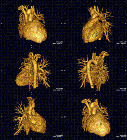
*Animated: Magnetic resonance imaging — placed from the Real G.E.N.E.R.A.T.I.V.E. course library (Geometry room). Source: Wikimedia Commons (via Wikipedia article media). [Details & license](https://commons.wikimedia.org/wiki/File:PAPVR.gif).*
> Magnetic resonance imaging (MRI) is a medical imaging technique used in radiology to form pictures of the anatomy and the physiological processes inside the body. MRI scanners use strong magnetic fields, magnetic field gradients, and radio waves to generate images of the organs in the body. ([Wikipedia](https://en.wikipedia.org/wiki/Magnetic_resonance_imaging))
<!-- REAL-GENERATIVE-MEDIA:END -->
<!-- LOCAL-MEDIA-PASS:START -->
## From the vault media library
!Magnetic resonance imaging thumb.png
*Magnetic Resonance Imaging — from the vault's own media holdings, placed 2026-07-09. MTN / Wikitube.io original · CC BY-SA 4.0.*
<!-- LOCAL-MEDIA-PASS:END -->
## Media (PD/CC)
<!-- MEDIA-DEPLOY:Magnetic_resonance_imaging/PAPVR.gif -->
!Gif Library/Magnetic resonance imaging/PAPVR.gif
*PAPVR.gif · Jccmoon at English Wikipedia · CC BY 3.0 · [source](https://commons.wikimedia.org/wiki/File:PAPVR.gif)*
<!-- /MEDIA-DEPLOY -->
<!-- SIGN-SYSTEMS:START -->
**Semiotic universals** (the notations and alphabet letters this article speaks — each opens its canonical card): resonance · spectrum · gradient · signal · flow. Index: the glyph gallery · SEMIOTICS PORTAL.
<!-- SIGN-SYSTEMS:END -->
> **Room:** [[Helium]] · **Status:** ✅ shipped
## Overview
**Magnetic resonance imaging** (MRI) is a non-ionizing tomographic imaging technique that maps the spatial distribution and relaxation behaviour of nuclear spins — overwhelmingly the **hydrogen-1 [[Proton|proton]]** in tissue water and fat — to produce cross-sectional images of soft tissue with contrast unmatched by any other modality. It rests on [[Nuclear_magnetic_resonance|nuclear magnetic resonance]], discovered independently by Bloch and Purcell in 1946 (Nobel 1952), and on the gradient-encoding insight of Lauterbur (1973) and Mansfield (1977, Nobel 2003) that made image formation possible. In a uniform field **B₀**, protons precess at the Larmor frequency **ω₀ = γB₀** (γ/2π = 42.58 MHz/T for ¹H), giving 63.87 MHz at 1.5 T and 127.7 MHz at 3 T. A resonant RF **B₁** pulse tips the equilibrium magnetisation into the transverse plane, where it decays with time-constant **T₂** while recovering longitudinally with **T₁**; pulse-[[Sequence|sequence]] design — spin-echo, gradient-echo, inversion-recovery, EPI, BOLD — selectively weights the resulting [[Signal|signal]] by T₁, T₂, T₂*, proton [[Density|density]], [[Diffusion|diffusion]], perfusion, or flow. Linear gradients **G(t)** encode position in the Fourier-conjugate **k-space**; image reconstruction is the inverse 2D/3D Fourier transform of the acquired data. Clinical scanners use a superconducting NbTi solenoid bathed in [[Liquid_helium|liquid helium]] at 4.2 K, gradient coils delivering 30–80 mT/m, and tuned RF transmit-receive coils. Applications span neuroimaging, musculoskeletal, oncologic, cardiac, breast, abdominal, fetal, and functional brain imaging — without ionizing radiation.
## See also
- Room hub: [[Helium]]
- p5.js Editor conventions: P5 JS EDITOR
- Wiki root: MAIN
---
*Scaffolded by `generative-microsim` from row 87 of the Helium sheet on 2026-05-12T09:33:10Z.*
<!-- REAL-GENERATIVE-MEDIA:START -->
<!-- CRAFT-LINK:START g12 -->
*Built to the [[WT!P5_js_Microsim_Master_Class|p5.js Master Class]].*
<!-- CRAFT-LINK:END -->
<!-- SPINEPATH:BEGIN g20 — shortest chain of Wikipedia links between local articles to a Compendium Main article; do not hand-edit inside -->
*Connected to the Apex Spine:* Magnetic resonance imaging → [[Properties_of_water|Properties of water]] — [[WT!Thury_Hydrodynamics_Compendium|Compendium]] section 6, *Water*.
<!-- SPINEPATH:END -->
## Wikipedia : Wikitube
**Strict pair:** [Wikipedia](https://en.wikipedia.org/wiki/Magnetic_resonance_imaging) : [Wikitube](https://en.wikitube.io/wiki/Magnetic_resonance_imaging)
## Previous hub tags
Tree parent: [[Helium]].
Legacy hubs: none.
---
*Sources: 1 legacy note. Minted wave 1, 2026-07-30 (v1.6 order).*